3   TRACE Instrument Guide

The Instrument Guide is intended to give the user an outline of the TRACE instrument and spacecaft, and to convey some of the salient points relating to the instrument that may be of assistance when analysing the data. It is by no means the only source of this information. The TRACE instrument (Section 3.1) is described in considerably more detail in Handy et al. (1999). Aspects of the instrument properties and calibration (Sections 3.2 and 3.3) are described in a number of calibration notes (see the list in Section 3.5). The C IV diagnostic capabilites of TRACE (Section 3.4) are described in Handy et al. (1998).

3.1   The TRACE Observatory

3.1.1   Instrument Description

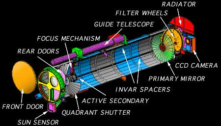
The TRACE instrument consists of a 30 cm diameter Cassegrain telescope and a filter system feeding a CCD detector (see Figure 3.1). Each quadrant of the primary mirror is coated for sensitivity to a different wavelength range. Since the four coatings share a common substrate, images in all ranges are co-aligned well. The corresponding quadrants of the secondary mirror are coated in a similar manner. All four mirror quadrants have multilayer coatings, which serve to define the passbands at each wavelength. Entrance filters exclude all visible Light and most of the energy in the UV - this help reduces scattered light and the heat load inside the instrument. A pair of filter wheels contains filters to select particular UV spectral regions. The 1024×1024 pixel CCD camera was developed for the SoHO/MDI program. An image stabilization system drives an active secondary mirror to compensate for spacecraft pointing jitter to a level of 0.1^¢¢. A data handling computer performs basic image manipulation and compression in order to reduce telemetry requirements.

Light entering the instrument passes first through the entrance filter assembly which transmits only far and extreme UV. Visible and near UV radiation (and hence most of the solar energy) are reflected back into space. Radiation transmitted through the entrance filters passes to a quadrant selector wheel that blocks three quadrants of the aperture so that only one quadrant of the telescope is illuminated at a time. Photons passing the wheel's open quadrant proceed to the primary mirror, encountering a multilayer coating for a narrow-band EUV quadrant or a broad-band coating for the UV quadrant.

The reflected beam from the primary mirror proceeds to the secondary mirror which reflects it towards the focal plane. The secondary mirror is active to correct for pointing jitter and has coatings matching those on the four quadrants of the primary mirror - it is also stepped to adjusted the focus of the different TRACE channels. The converging beam from the secondary mirror passes through the central hole in the primary mirror where it encounters two filter wheels in series.

Each four-position wheel has three filters and one open position (see Tables 3.1 and 3.2). The two wheels contain thin film aluminum filters for use with the EUV channels, and four UV filters. A thin aluminum (EUV) filter is located in each wheel for use in series if pinholes in both of them become a problem. This has not been necessary and the baseline/front filter has always been used thus far. The Lyman-a filter (1216 Å) is deposited on a magnesium fluoride substrate and the remaining UV filters are on quartz substrates. A narrow band UV filter for the C IV lines at 1548 and 1550 Å is deposited on crystalline quartz (as is a narrow band filter peaking at 1570 Å). The filter for the continuum at 1600 Å is made with the same deposition coating on a fused quartz substrate. This substrate sharply attenuates the C IV lines and makes it possible to subtract the longwave transmission of the 1550 Å narrow band filter. Normally one filter wheel is set at open; the other selects the spectral region. To observe in the 5000 Å band, one filter wheel is open and fused-silica is selected on the other.

Radiation passing the filter wheel assembly next encounters the focal plane shutter. The shutter mechanism consists of a disk mounted directly on the shaft of a brushless DC motor. Two apertures are provided in the disk, wide for exposures longer than 20 msec and narrow for exposures that are multiples of 1.6 ms. The final element in the optical train is the Lumogen-coated CCD camera. Its 21 micron pixels each subtend 0.5×0.5^¢¢ at the focus of the telescope. Ray traces of the optical system show that optical aberrations are smaller than one pixel throughout the field of view, even with maximum secondary mirror tilt.

3.1.2   Spacecraft Orbit, Attitude Control and Pointing

TRACE is a 3-axis stabilized, Sun-pointing spacecraft. It is in a Sun-sychnronous (98^°) orbit of 600×650 km.

The TRACE attitude control system (ACS) includes three reaction wheels, three electromagnetic torquers, a 3-axis magnetometer, a gyro system, coarse sun sensors, and a fine sun sensor. High sensitivity pitch and yaw error signals are provided to the ACS by the TRACE Guide Telescope. The ACS uses these signals to limit pointing jitter to < 20^¢¢; the Image Stabilization System (ISS) removes residual jitter using higher frequency signals from the guide telescope.

Within the guide telescope, a pair of independently rotatable wedge prisms mounted between the entrance filter and the objective lens allows the optic axis of the telescope to be deflected in any direction within a cone of 1 degree half-angle centered about the optic axis of the main telescope. The spacecraft is maneuvered by offsetting the optical axis of the guide telescope such that the main telescope points to the desired portion of the solar disk.

The ISS drives the active secondary mirror to compensate for spacecraft pointing jitter to a level of 0.1^¢¢. It is an open-loop control system in the sense that the error signal is derived from the guide telescope rather than from motion of the image in the main telescope.

TRACE does not use a star tracker. The roll axis is defined using Earth's magnetic field; the gyro system provides error signals for roll stabilization. Steady slow drifts in roll (~0.7 degree/hr) can be accepted without degrading the science.

3.2   TRACE Instrument Properties

3.2.1   CCD Camera

TRACE uses a flight spare CCD from the SoHO MDI instrument - it was designed by Loral for MDI. It is a 1024×1024, 3-phase, Multi-Phase Pinned (MPP), 21 micron pixel design which incorporates dual serial registers for redundancy; is front-illuminated, and is not thinned. The pixels each subtend 0.5×0.5^¢¢ at the focus of the telescope.

The CCD is phosphor-coated to give it UV sensitivity. The material used was Lumogen, made by B&K, and deposited by Lorel. The sensitivity of the Lumogen-coated CCD is about 0.08 at the EUV wavelengths, 0.09 at 1216 Å, 0.15 at 1600Å, and ~0.40 in the visible. The system gain of the camera is ~12 electrons/Data Number (DN) when using the A amplifier (which is normally the case); the B amplifier system gain is ~45 electrons/DN. The response of the camera is very linear with exposure; weak pixels are also linear.

The 12-bit ADC tops-out at 4096 counts - count levels in excess of this return this value. This represents only 20% of the full-well capacity of a pixel, so unless the countrate is extremely high there is little spreading from (ADC) saturated pixels.

The CCD is designed to operate at temperatures below -55 ^°C. It is cooled by an aft-facing passive radiator system located at the rear of the spacecraft. The detector runs cold to reduce dark current, and mitigate radiation damage effects.

The peak data rate of TRACE is theoretically limited by the time taken to read the CCD, and practically limited by signal level considerations. The amount of time required to obtain a 1024×1024 image is determined by the CCD read rate of 500 Kpixels/s to be 2.2 seconds. N×N subarrays can be read out faster by a factor of almost 1024/N; there is usually some fixed ``overhead''. On-chip summing and/or binning of pixels in the image processor can be used to invoke compromises of spatial resolution, FOV, signal level and peak image rate. The 12-bit pixels are compressed in cells using a JPEG algorithm.

3.2.2   CCD Detector Properties

Flat field correction maps have been derived but show little departure from unity - for white light typical excursions across the field show ~1.5% peak-to-peak. To date, the flat field correction are not applied.

Calibration images of the CCD dark-current are taken roughly every two weeks. The dark current is essentially zero (~0.1 DN/sec), has changed little during the mission, and varies slightly with temperature. The routine trace_prep presently uses a fixed dark current for all exposures, but will soon use a temperature dependant value.

There is a readout pedestal on the CCD of almost 87 DN (in non-summing mode). This varies for different summing modes and when different parts of the CCD are readout (e.g. the middle 256×256), but is not dependent on exposure time. It increases in magnitude and becomes less uniform over the CCD with progressively higher summation modes (2×2, 4×4, 8×8). The pedestal decreases slightly as the temperature increases. The routine trace_prep presently removes a fixed pedestal but will soon use a temperature dependant value.

The CCD readout noise is typically less than 2-3 DN/sec. This is probably electronic in origin and includes a herring-bone pattern on the image. The pattern is modulated by vertical stripes that may be caused by the CCD maufacturing process. CCD readout noise is discussed further in the section on image quality.

The TRACE CCD experiences a lot of problems with orbital background (i.e. SAA and HLZ's). The effect is greater than was anticipated before launch for HLZ's and data are no longer taken in the (longer exposure) EUV channels when TRACE is in the radiation belts. The problem takes the form of spikes or tracks left in the CCD image. The effects of orbital background are discussed further in the section on image quality (see Section 3.2.7). The approximate timing of passages through the belts can be determined from the fdss files (see Section 2.1.2).

3.2.3   Image Coordinates and Pointing

The pointing coordinates included in the TRACE index records are for the White-light channel. The EUV channels, and the UV Lyman-a (1216 Å) channel, are offset slightly from the white light and other UV channels - a set of measured offsets is given in Table 3.3. For alignment with data from other instruments, the index record needs to be adjusted - this is done by the routine trace_wave2point.

Because of slight differences in the optics, it is necessary to change the focus between exposures for the different TRACE channels - an adjustment of ±5 mm in the position of the secondary mirror is provided for this purpose. The focus of each channel has been determined since launch by imaging solar features with fine structure at several focus adjustment positions and determining the best focus by examining the sharpness of each image - e.g. solar prominences were used for the 1216 Å channel. Note, a new set of inter-channel offsets has been derived for the new set of focus positions adopted on September 24, 1998 - these are given in Table 3.3. The new focus adjustment positions brings the 1216 Å channel closer to the positions used for the other channels than was the case prior to then.

The pointing accuracy of TRACE is probably good to 5-10^¢¢ - this may improve when a better wedge calibration is available. The pointing stability within a stream of images is very good - better than a few tenths of a pixel. Movements of the quad-shutter causes a ~4^¢¢ disturbance that takes a few seconds to damp down, and can leave a residual change of 0.5^¢¢ or less.

There is a small pointing wobble over the course of an orbit, of the order ±1^¢¢. This correlates well with temperature and may be caused by a slight flexing between the guide telescope and the main TRACE telescope; it will be removed by the analysis software once it has been characterized. In movies, an apparent pointing drift can occur if the roll of the spaceraft is not properly aligned to Solar north-south - a 1^° error in the roll axis would represent 17^¢¢ at the limb. Since TRACE does not have a star tracker, data from the SOHO/MDI instrument are needed for an absolute roll calibration.

Although TRACE collects images over a 8.5×8.5 arcminutes field-of-view (FOV), the images are vignetted by the telescope optics. The vignetting is caused by the filter-wheel, is not symmetric about the center of the FOV, and is different for each channel because each uses a different mirror quadrant. For the UV passbands, since the same mirror quadrant and filter wheel position are used, the vignetting should be the same for all channels, although the different focus position for the 1216 Å channel has some effect.

3.2.4   Image Exposure and AEC

TRACE often uses a simple Automatic Exposure Control (AEC) algorithm, very similar to its predecessor on Yohkoh/SXT. The algorithm adjusts the exposure index based on a 128-bin histogram of the previous CCD image, which is taken after the removal of bad pixels and the CCD readout pedestal. For most applications, the AEC is programmed to maximize dynamic range while avoiding saturation of the CCD. Simply stated, the approach is to choose the greatest exposure time that will not saturate pixels in the highest percentile of intensity. AEC behavior is controlled by several adjustable parameters which are stored in the AEC table - this contains entries for each wavelength and target class that define thresholds and amounts by which the exposure should be adjusted in case of over- or under-exposure.

Details of the TRACE Automatic Exposure Control algorithm, including a description of the parameters used to control it, can be found on the TRACE Web pages at MSU.

3.2.5   Image Timing

The image time downlinked in telemetry is the time that the shutter closes. The start of the exposure can be determined by subtracting the exposure time. There is an uncertainly of ~0.1 secs in the timing.

3.2.6   Image Resolution

The plate-scale of the white-light TRACE images have been determined by J.-P. Wuelser to be:

The plate scale is thought to be effectively the same for all channels, if they are in focus. The resolution of TRACE is therefore very close to its planned 1^¢¢.

3.2.7   Image Quality

TRACE uses a modified 12-bit JPEG algorithm for data compression. The algorithm has a nearly lossless mode that preserves 12-bit data with a maximum error of 1 count and a wide range of lossy options which are tailored to different image characteristics. The image is compressed in cells of 8×8 pixels - these can clearly be seen if a decompressed TRACE image is closely examined.

In itself, JPEG compression affects an image in a manner that is well understood, but for TRACE there are some additional effects described below:

Orbital Background
The TRACE CCD is significantly affected by orbital background (i.e. the SAA and HLZ's). The problem takes the form of spikes or tracks left in the CCD image. It is most acute with the long exposures in the EUV channels; the shorter exposures of the UV channels are much less affected. Because the spikes are not removed on-board, the intensity distribution of the spike is spread by the JPEG compression leaving a residual signature that is hard to quantify and which affects the accuracy of the diagnotics.

CCD readout noise
The CCD image is affected by readout noise that is probably electronic in origin. It takes the form of a herring-bone pattern on the image; the pattern is modulated by vertical stripes that may be caused by the CCD maufacturing process. Although its amplitude is small (typically 2-3 DN), the noise creates spikes in the image FFT; this can be removed with Fourier techniques.

Filter Mesh Diffraction Pattern
TRACE uses a standard design entrance filter in which the support mesh is an electroformed metal fashioned as a regular grid of fine wires in a rectangular pattern. This mesh acts as a diffracting element, which has a regular, well characterized pattern in the focal plane. It is most noticable if a bright, compact flare kernel is in the TRACE field of view. The pattern can be removed during data analysis by straight forward Fourier techniques. A detailed study of the diffraction pattern is available under the instrument section of the TRACE Web pages at Lockheed-Martin.

Atmospheric Absorption
For several weeks either side, and while TRACE is in its eclipse season, the signal observed by TRACE is attenuated by the Earth's atmosphere during parts of its orbit and the response of the EUV lines is compromised. This effect is present in each orbit for several minutes either side of the actual eclipse (see Appendix B.4). While the images are still fine for morphological studies, they should only be used for diagnostic purposes with extreme caution.

3.3   TRACE Instrument Response

3.3.1  Sensitivity

The characteristics of the TRACE channels are given in Table 3.4, where the sensitivity is defined as:

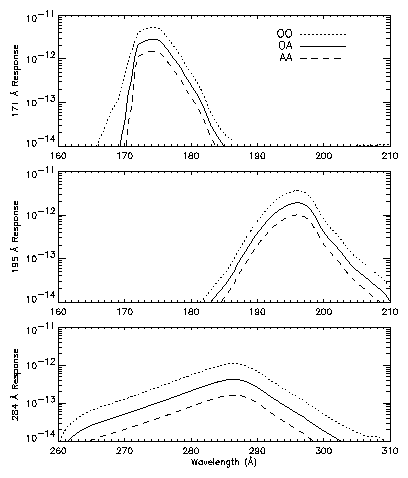
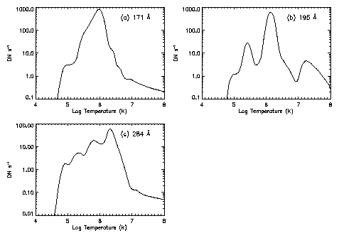
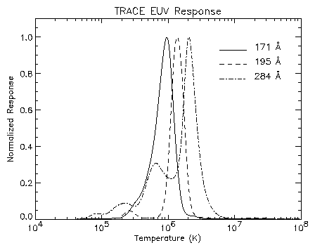
The wavelength response of the TRACE optical and UV channels is shown in Figure 3.2, and of the EUV channels in Figure 3.3. The temperature response of the TRACE EUV quadrants are shown in Figure 3.4.

Details of the manufacture of the TRACE mirrors and filters, and the sensitivity of the TRACE channels, and the calibration of the instrument are given on the TRACE Web pages at SAO and Lockheed-Martin.

3.3.2   On-orbit characterization of the Flat Field Response

On-orbit flat fields of the TRACE CCD and optics in WL and 1700 Å wavelengths have been generated using the the Kuhn-Lin flat-field algorithm. This algorithm uses a number of images at slightly shifted locations on the CCD, with the images out of focus to reduce contrast.

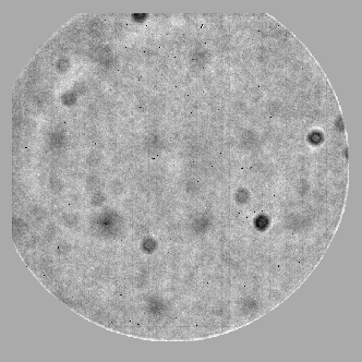
The WL flat field is quite flat and of good quality (in the sense that it corrects WL images to high accuracy). The flatness and quality has changed very little since launch, with a difference image of two flat fields taken 7 months apart showing ±1.0% peak-to-peak variations, the same range as the flat fields themselves.

Several features are evident in the WL flat field of Figure 3.5a. There are many small dark spots of ~1-3 pixels across with intensities of 20-80% of the normalized field. These were present on the CCD prior to launch and correct well in the WL images. Because the spots interact poorly with the JPEG data compression algorithm, most of them are treated on-board as bad pixels and are replaced by a good nearest neighbour.

Larger spots (~50-60 pixel diameter with an intensity of ~96-98%) are also evident on the WL flat field. These are most likely shadows of dust particles on the fused silica filter in the aft filter wheel. They disappeared when a WL flat field was generated from images that did not use the fused silica filter. In these flat fields, another set of larger (~80 pixels), less well focused, and lower contrast (~97-99% intensity) spots became apparent as a regular array on the CCD. This array was seen at several wavelengths during CCD testing prior to launch and is believed to be a CCD fabrication artifact. All of these features correct well in the WL images.

A pair of bad partial rows (CCD columns actually) are visible in the WL flat field. In addition, vertical and horizontal dark lines are seen every 24 pixels at very low contrast. These are a CCD fabrication artifact.

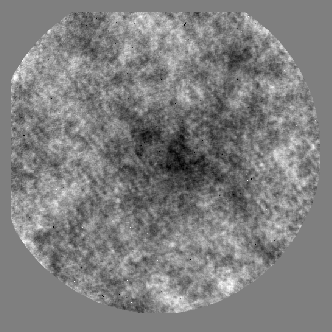
The flat field at 1700 Å (Figure 3.5b) shows some degradation in the relative response across the field of the CCD in the center. Although 30 images were utilized in the analysis of the flat field, most of the CCD structure is not resolved at this wavelength due to higher contrast, lower count rates, and changing structure in the original images when compared to those in WL. Despite defocusing, the 1700 Å images in quiet sun have network features three times brighter than average intensity. However, the pair of bad partial pixel rows observed in the WL flat field is also present in the 1700 Å flat field.

The 1700 Å flat field for 7 January 1999 demonstrates a degradation of about 5-8% in the center region of the CCD with a small portion degrading up to ~10%. A 1700 Å flat field from 9 October 1998 displayed about a 2-5% relative degradation in the same region. This relative degradation in response across the field is probably occurring in the Lumogen coating on the front of the CCD. A similar loss has been noted near the CCD center in EUV images of loops on the limb when compared to images with the limb moved to regions near the outer, non-degraded portions of the CCD area. The decrease in Lumogen sensitivity near the center of the CCD is probably a result of damage by the accumulated EUV dosage. However, the degree of degredation is less than was anticipated.

Efforts are ongoing to generate satisfactory flat-field images for the other lines. The EUV wavelengths are particularly resistant to this method, as they are of extremely high contrast with much of the image at a very low count rate. Flat field data taken in the 171 and 195 Å channels in May 1999 suggests that the degredation in sensitivity in the EUV is similar to that at 1700 Å.

For the most recent information on flat field measurements, see the TRACE Web pages at Lockheed-Martin.

3.4   TRACE Diagnostic Capabilities

TRACE can provide information on the morphology of the magnetic field directly from its images and can also provide a number of other diagnostics.

When TRACE is in or near its eclipse season, care should be taken when using data for diagnostic purposes because of the effects of atmospheric absorption - see Appendix B.4.

3.4.1  Temperature

The three EUV channels overlap in temperature coverage and can be used to investigate the temperature of the coronal plasma. As all the EUV wavelength bands are dominated by different ionization stages of iron, ratios do not depend on a knowledge of iron abundance. The band ratios are extremely sensitive to temperature changes, varying by factors of up to 40 over typical coronal temperature ranges. This compares favorably with broad-band temperature diagnostics (e.g., factors of 2-4 for Yohkoh/SXT temperature ratios).

Figure 3.6 shows the relative contributions of the three EUV bands. Ratios of the bands are multivalued and are ambiguous for certain temperatures. Obtaining images in all three EUV channels can help to resolve the ambiguity if the plasma is nearly isothermal. In practice, this is only likely to work if careful background subtraction is done. Without background subtraction, temperature ratios yield inconsistent or nonsensical results in nearly all cases.

It is surprisingly easy to derive differential emission measure distributions from TRACE data, primarily because there are few channels and so an inversion by linear techniques is well-behaved. There are, however, several pitfalls:

1) The DEM is meaningful only under the assumption that most of the emission measure is in the range 0.4-3 MK. Thus, it is applicable mainly to non-flaring active regions, quiet sun, and polar plumes.

2) There are only three channels, so the DEM must be composed of just three basis elements. The choice of basis can have an effect on the properties of the result.

3) The resulting DEM curves are not always positive for all temperatures. This may result from excessive noise (if the DEM is done for a single pixel) or simply a choice of basis that is ill-suited to representing the actual temperature distribution. Integration over tens or hundreds of pixels will virtually always yield a positive DEM.

3.4.2  Emission Measure/Densities

3.4.3  Observing C IV Lines

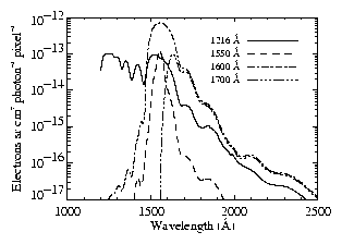
TRACE uses a set of three filters to observe and correct the C IV images (Handy et al, 1998). The filters characteristics are:

1) 1550 Å filter - 30 Å FWHM, centered at 1550 Å. Observes C IV + C I, Fe II lines + continuum.

2) 1570 Å filter - 30 Å FWHM, centered at 1570 Å. Observes C I, Fe II lines + continuum.

3) Continuum only - Same interference coatings as 1), but made on a substrate that rejects light below 1700 Å.

Reduction of a set of three observations uses simple matrix methods. Let P(i) represent the image made with the ith filter. Let I(j) represent the intensities of the C IV lines (j=1), the chromospheric contribution (j=2) and the long wavelength continuum (j=3), respectively. Then the matrix representation of the set of images is:

[P] = [A][I]

where [P] and [I] are column vectors and [A] is the matrix A(i,j) representing the transmission of the i th filter to the j th wavelength. The formal solution is:

[I] = [a][P]

where [a] is the inverse of [A]. The transmissions A(i,j) is measured during instrument calibration; the matrix solution is expected to be well behaved because of the nature of the problem. (Note that A(3,1) and A(3,2) are both zero and that A(l,j) and A(2,j) are linearly independent because of the way the filters are designed).

The reduced observations provide images of the chromosphere (from the C I and Fe II lines) as well the transition zone. The long wavelength continuum image is probably formed somewhere between the high photosphere and the temperature minimum, based on the work of Foing (1986). Finally, images taken through the UV entrance filter only are dominated by wavelengths near 2500 Å, which arises in the photosphere. These images are used extensively for co-alignment with SoHO and other observations.

3.4.4  Aeronomy

See Aiken et al., 19?? for more information on this type of science.

3.5   References

TRACE Investigation and Technical Plan (Phase III & IV), August 1994, LMSC P017270P-1
``The Transition Region and Coronal Explorer'', 1999, Handy et al., Sol. Phys., in press.
``UV Observations with TRACE'', 1998, Handy et al., Sol. Phys., 183, 29
``Thermospheric Molecular Oxygen??'', 19??, Aiken et al., ???.