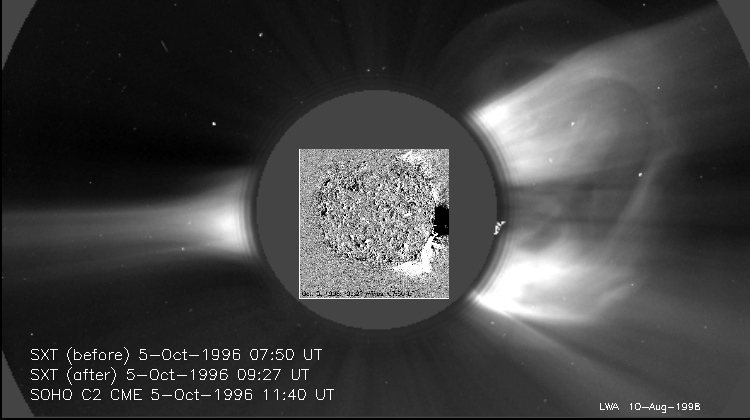
We interpret the image as follows: a flare occurred far around on the invisible hemisphere; it resulted in X-ray dimming visible as the dark area on the inset SXT image at the W limb. This showed the origin of some of the CME material that came spewing out, as shown in the outer (LASCO) image. The X-ray image shows brightenings both north and south, suggesting that the overall restructuring dropped energy into these quadrupolar features. Somebody should write a paper about this image!
y(T) = d(nineV)/dT.
Solar physicists spend much happy time debating about the relevance of DEM, as opposed to the simpler assumption that everything is isothermal. This latter is usually not as stupid an approximation as it sounds, but of course in principle it is always wrong. But how wrong? This nugget describes a well-controlled theoretical situation where we know that the source is multi-thermal, and what its geometry is. Let us use this example to see how much it would change our naive intepretation of the Yohkoh SXT observations.
 |
 |
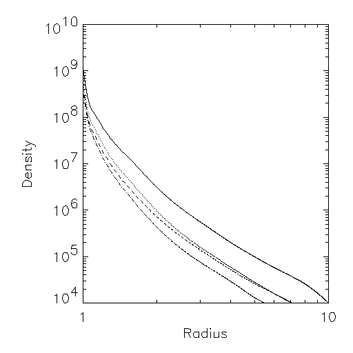
Withbroe models in decreasing order of peak temperature:
|
First, the DEM itself: This is a function of the impact parameter of the line of sight through the corona. Impact parameter zero would be an integration straight into the geometric center of the Sun; unity would be just tangent at the limb; a value 1.5 would have a projected height of half a solar radius above the photosphere. Here are these three cases:

These DEM's clearly have distributions in temperature (the X-axis, in units of millions of K), so we would expect the SXT response to differ from (say) the isothermal model evaluated at the projected height (for impact parameter > 1); for a view straight down at disk center, the effective SXT temperature will obviously be larger than the temperature at the very "base of the corona", since the model temperatures increase monotonically with height initially. But how much larger is this systematic error in the measurement?
In the plots above, the Y-axis has known but somewhat irrelevant units. But of course the values for 1.5 radii are small - the X-ray corona rapidly becomes dim for larger impact parameters. The bias in temperature varies with height for these models.
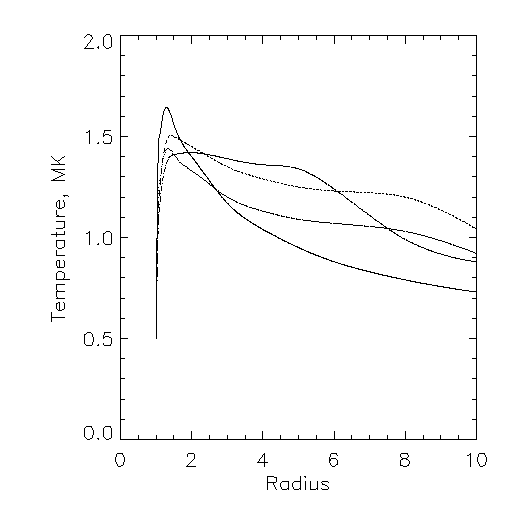
The vertical case is unique: by using the DEM in the plot on the upper left, we find a maximum effective temperature of TT1, for Withbroe model N1 ("quiet corona"), and a minimum temperature of TT2 for model N2 ("polar hole, minimum"), which seems plausible. Both of course greatly exceed the temperature of the base of the corona in the models, since hotter material at higher altitudes contributes to the integration.
As a function of impact parameter, we get the following plots of the temperature error resulting from the DEM consideration:
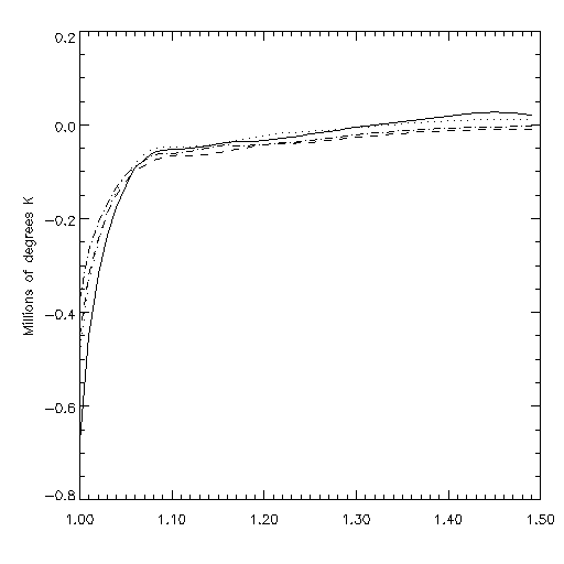
where the different line styles show the four different Withbroe models. We see a systematic discrepancy, but it's less than 0.1 MK above 1.05 solar radii for all cases. Near the Sun, the apparent temperature is always higher than the true plane-of-the-sky temperature because the line of sight samples higher altitudes, and the temperature increases with height in this region of the models. It's hard to say how seriously to take this - the Withbroe models, now senior citizens in the coronal-modeling effort, probably have large errors at low altitudes anyway. On the other hand there are no recent comprehensive models that I'm aware of - let me know if they exist, and I'll re-do this analysis.
We don't find extremely large temperature discrepancies, but they are significant (or should be so) to coronal modelers. The line-of-sight integration over models of this type results in an observational bias. It's an illustration of how one characterizes such a bias, which many astronomical observations unfortunately must deal with, by using a "forward-method deconvolution". The alternative to this, a mathematical inversion of the data to produce two model-independent functions (density and temperature) is beyond the talents of the author, but there are people out there who probably can do it.
I know that these plots are tedious by comparison with our beautiful pictures, but... we need to be quantitative!