
Notes for observing with the UVOT UV Grism
Last updated: 26-July-2016: updated to conform to the 2015 calibration
The Swift UVOT UV grism can provide 1700 - 5200 Å spectra of modest S/N and spectral resolution R ~ 150 for stars in the magnitude range 9.5-14.5. The first order UV grism spectrum is not contaminated by second order emission below 2750 Å, and depending on where the spectrum falls on the detector and the brightness of the UV, the second order overlap starts at longer wavelengths. Note that the V grism is sensitive down to 2900 Å, and is actually more sensitive than the UV grism for the longest wavelength UV light (2900-3200 Å).
The wavelength calibration of the UV grism has been difficult because the spectra show a curvature and sensitivity that varies with detector position. In the middle the curvature is minimal and first and second orders overlap. On the top of the detector the second order shifts and lies next to the first order. In the lower half the second order lies partly over the first order, shifted by a lesser amount in the opposite direction. Because the UVOT pointing is only accurate to a few arcminutes, with improved repeat positioning to within a few arcseconds using a “slew in place” (“SIP” in Swift terminology), there can be variations even within consecutive exposures. Details on the calibration and capabilities are laid out in the UVOT grism calibration paper by Kuin et al. (2015).
The following decisions need to be made when observing with the UV grism:
- Slew in place?: The pointing accuracy after an initial slew may be only 1 or 2 arcminutes. This uncertainty is not significant for GRB followups with direct images, but can critically affect the calibration of the UV grism data, since there are significant wavelength and sensitivity changes across the detector. The use of a second slew after the arrival at the target (a “slew in place”) can reduce the pointing uncertainty to a few arc seconds (typically less than 20 arc seconds). However, if one is primarily interested in XRT data then one might not want to spend the extra ~3 minutes required to improve the grism observation by taking a slew in place. Note that often one tries to avoid observing with the grism during the first few and last few minutes of an orbit anyway (because the sky background is large) so the use of a slew in place does not affect the prime grism science time.
- Clocked or Nominal Mode?: Zeroth-order spectra only appear in the area covered by the grism, whereas first-order spectra can be dispersed off the edge of the grism. Thus, in principle, the use of clocked mode can minimise the contamination of first-order spectra by unrelated zeroth-order images. Unfortunately, for the UV grism the default clocking is insufficient to perform this separation for the UV first-order spectrum. However, clocked mode remains useful because it suppresses the total sky flux, and for that reason must be used in crowded fields (e.g. low Galactic latitudes). Clocked mode also has slightly better sensitivity (see below) and smaller spatial variations in wavelengths and sensitivity. One disadvantage of clocked mode is that it introduces vignetting and so spectra are retrieved over a smaller field, which may be important for extended sources or if a slew in place is not used. For sparse fields, the choice between clocked and nominal mode is often decided by which one gives a better roll angle for a particular observing date.
- Roll Angle: The contamination of grism spectra by zero and first order of unrelated sources depends on the roll angle of the observation. An IDL grism simulator (restricted to the default position; no offset) is available at http://idlastro.gsfc.nasa.gov/ftp/landsman/simgrism/ which displays a DSS image with simulated dispersed spectra for a given roll angle. (This software can be run under the IDL virtual machine, without an IDL license.) For a given observing time, the planners have very limited flexibility in choosing the roll angle. However, the simulator can be used to select a range of good observing dates or to choose between clocked and nominal model. In very crowded fields, splitting the observation between to roll angles 2-3 degrees apart can help identify weak contaminating zeroth orders.
- Offset position: Using an offset in the clocked mode can reduce or remove the contamination from the second order and reduce the background in the uv part of the spectrum. For example, an offset of +5.6 arc minutes in detector Y position (zero in X) will position the spectrum close to the occulted zeroth orders boundary and will thus need a slew-in-place. Usually contamination by zeroth orders is reduced significantly above 2000 Å. Small offsets (+1-3 arcminutes in Y) to the top part of the detector are discouraged as there are a few pixels whose sensitivity is up to 30% less which is thought to be due to small dust particles in the light path to the detector. [see the SSS map in the CALDB] Offsets need several days of planning. Therefore, offsetting the source in an observation can not be done in a Target of Opportunity observations if the observation needs to be done in the next 3-5 days. If a spectrum is needed right away, it needs to be uploaded as a modification to the plan, without a “SIP” and may fall anywhere in the central area.
- Exposure time: The effective areas, for zero coincidence loss, for the UV grism in the nominal and clocked modes at the target position is given in the table below. Note that this effective area is for computing the count rate integrated perpendicular to the dispersion, and that the dispersion varies from about 2.0 Å/pixel near 1800 Å to about 3.5 Å/pixel near 3000 Å. The “Cts/s” column gives the predicted counts/s (per pixel integrated perpendicular to the dispersion) for a faint and a brighter source with a flat spectrum (in erg cm(-2) s(-1) Å(-1)).
Table of UVOT Effective area (default position, 2015 calibration) and background-subtracted source count rates for constant flux sources (in ergs/cm2/s/Å:
| Wavelength | Nominal Effective | Nominal log f=15 | Nominal log f=12 | Clocked Effective | Clocked log f=15 | Clocked log f=12 |
|---|---|---|---|---|---|---|
| (Å) | Area cm^2 | C/s/bin | C/s/bin | Area cm^2 | C/s/bin | C/s/bin |
| 1700 | 2.4 | 0.03 | 32 | 1.4 | 0.06 | 55 |
| 1900 | 8.4 | 0.17 | 8.0 | 0.16 | ||
| 2100 | 10.7 | 0.2 | 11.8 | 0.22 | ||
| 2300 | 15.2 | 0.3 | 14.4 | 0.26 | ||
| 2500 | 16.4 | 0.4 | 16.3 | 0.34 | ||
| 2700 | 16.4 | 0.5 | [487] | 17.6 | 0.44 | [440] |
| 2900 | 15.4 | 0.6 | [620] | 17.1 | 0.55 | [550] |
| 3200 | 12.6 | 0.6 | [620] | 12.4 | 0.61 | [605] |
| 3500 | 10.2 | 0.6 | [670] | 10.5 | 0.63 | [635] |
| 4000 | 8.2 | 0.6 | [670] | 8.0 | 0.67 | [665] |
| 4500 | 5.5 | 0.6 | [600] | 5.6 | 0.56 | [565] |
| 5000 | 3.3 | 0.45 | [450] | 3.4 | 0.40 | [395] |
| 5500 | 1.3 | 0.3 | 265 | 1.9 | 0.18 |
Variability studies: The typical 1-3% error in the UVOT zeropoint has a large contribution from pixel-to-pixel sensitivity variations. In 2016 a WD calibration source was used to determine how accurate its flux can be measured in repeated measurements when the source falls on nearly (within 8 pixels) on the same place on the detector. These repeated photometric observations have been shown to differ by an error of less than 1%. This means that variability studies are generally limited by the accuracy of the zeropoints, or for the grisms, the accuracy of the flux calibration. Where high relative accuracy in a series of spectra is important, it is recommended to use the same position (offset) on the detector; requesting a (double) slew in place (“SIP”), and also make sure that the same roll angle is used. The reason for that is that the contamination due to weak background sources comprises the largest source of the flux error in the UV and using the same roll angle guarantees that the same background is present. In practice the range of available roll angles for a certain target changes over the year, giving a limit of the period over which this strategy can be employed. The pointing accuracy of Swift after a slew from another target is 1-2 arc minutes which can be improved using a SIP. Using a SIP costs extra time, and extra images will be taken that cannot be used in the variability study because those will not generally be at the same detector position. Of course, if there is a large variability (more than 0.05 mag) a SIP is not really needed. A double SIP is needed to constrain the position to within about 30 pixels (15”). Generally that is enough to increase the photometric accuracy, though source brightness and limited exposure time typically dominate the photometric error.
Background Count Rate: Observations of faint sources are dominated by the background count rate (taken as 0.3 cts/s/bin for the table), which must be considered when predicting the expected S/N. The sky background on a grism image increases with decreasing Galactic latitude, ecliptic latitude, Sun angle, and Earth limb angle. The background counts per second in a 13 pixel extraction slit roughly varies from about 0.4 cps at low Galactic latitude to about 0.2 cps at high Galactic latitude. (A 13 pixel extraction slit is roughly the smallest slit size that does not significantly reduce the source count rate and is close to the default size used in the 2014 UVOTPY python-based software). Consider the computation of the S/N at 2500 Å in a 2000s exposure of a high Galactic latitude source with a monochromatic flux of 10^(-14) erg cm(-2) s(-1) Å(-1) in the nominal grism mode. From the table on this page the expected source rate is 0.048 cps. The S/N then is S/sqrt(S+B) = (2000*0.048)/sqrt(2000*(0.2 +0.048)) = 4.3. The actual S/N will be somewhat lower because the background includes non-random noise due to the presence of faint stars and first-order spectra. The background is reduced in parts of the image for the clocked mode.
Software: The original “uvotimgrism” software in the “Ftools” package is NOT able to deal with coincidence loss corrections, nor the curvature in the UV grism, nor to correct for a different dispersion and effective area at offsets from the default position. The “Ftools uvotimgrism” program can still be used for spectra sources of medium brightness taken at the default position, and cometary observations. The old effective area is implicitly used and the unknown error in the flux likely is double that of the 2015 grism calibration of Kuin et al. (2015). UVOTPY, a Python-based spectra extraction for the Swift UVOT grisms which was developed along with the calibration has been made available and is recommended for most grism observations. The package is available at Github, while further grism calibration and software documentation is available at MSSL/UCL.
Effective Area: The effective area for all four grism modes can be examined here :`ref:fluxcal_v1. The thin curves sample different positions in the nominal mode on the detector. In the clocked modes the effective area varies more significantly by position, see Kuin et al. (2015). Note that although the UV grism can record a visible spectrum, the sensitivity is less than half that of the V grism, and can suffer significant contamination from second-order UV light.
Coincidence loss correction limits: For very bright sources the coincidence loss can no longer be corrected. This is discussed further here The coincidence area determination in the Grisms.
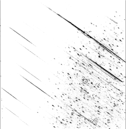
The appearance of the spectrum on the image will show increasing patterning around very bright lines, for example consider the bright spectrum line in the top spectrum in the figure below.
figure 1: UV grism (clocked mode) image
Caveats
Some considerations to be aware of when using the UV grism
- A single grism spectrum shows a fixed pattern noise that is only partially suppressed by
applying a mod-8 correction because of ever present coincidence loss. It may be useful to combine spectra whose positions on the detector rarely are identical to further suppress this fixed-pattern noise.
- Near very bright spectral lines close or above the brightness limit for coincidence loss
correction, the surrounding data points are affected by strong coincidence loss over ~50 Å while the line shape narrows at the same time. The line-narrowing does not occur for lines that do not suffer much coincidence-loss.
- Grism spectra do not have an absolute wavelength scale. Two methods are in use to define
an ‘anchor’ to the wavelength scale using either the zeroth order positions, or a mapping from the source position taken in a lenticular filter right before or after the grism exposure. When using the centroid of the zeroth order, since the zeroth order is itself dispersed, the position of the anchor point may vary with spectral shape. In addition, strong mod-8 noise may shift the position of the centroid. Finally, the zeroth order (which contains both UV and visible light) is often saturated. So there may be a zero point shift of about 4 pixels (leading to an uncertainty of 10 Å in the UV grism spectrum).
- The aspect correction based on the positions of the zeroth orders in the image sometimes
fails in which case the error may be very large. Using a lenticular filter image position, who have good aspect corrections, the accuracy is also typically 4 pixels. However if the spacecraft pointing drifts between exposures, which can be significant in some sparse starfields with non-optimal lock of the star-trackers, the error in the wavelength anchor again can be significantly larger. From exposure to exposure the anchor offset generally varies. Not all grism calibration files are presently in the Swift CALDB; the later ones are distributed with the UVOTPY software.
Example Spectra
Examples of UVOT UV grism spectra are shown below.
Figure 2:
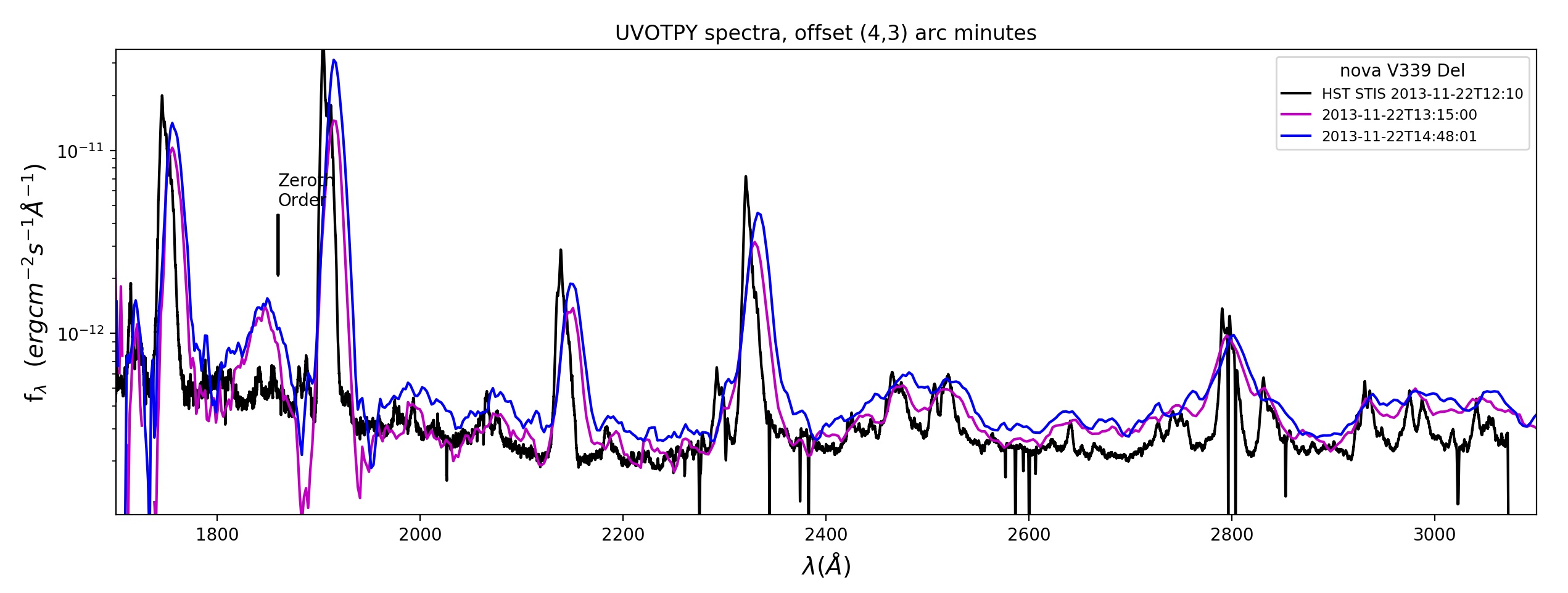
Figure 2 shows nova V339 Del in outburst (V ~ 11.0) in November 2013 (day 101 in the outburst). This spectrum shows N III] 1750 Å emission which is near the extreme wavelength limit of the UV grism sensitivity (1700 Å). Two exposures were taken by UVOT around the time of a spectrum taken by the STIS instrument on the Hubble Space Telescope. A zeroth order of a background source contaminates the UVOT spectrum around 1850 Å. The UVOT flux in the brightest lines needs a substantial coincidence-loss correction, and the flux is seen to be higher in the UVOT spectra which is likely due to the known variability of the nova. No correction for the wavelengths has been made after extraction of the spectra by “UVOTPY”, and a shift of about +7 Å can be noticed.
Figure 3:
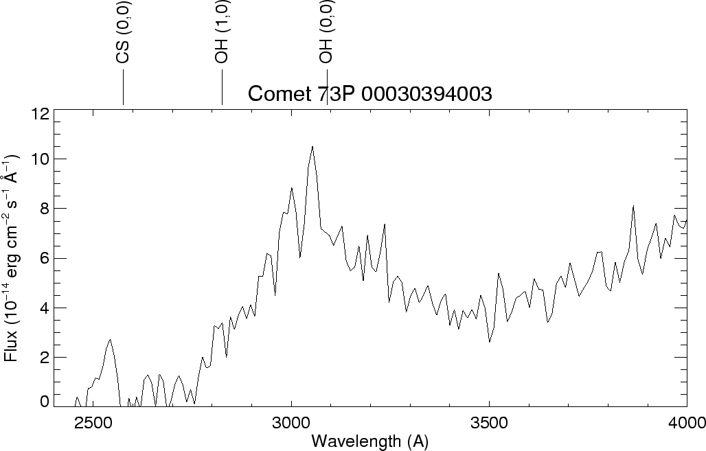
Figure 3 is a spectrum extracted with the “Ftool uvotimgrism” of the comet 3P/Schwassmann-Wachmann obtained in April 2006 showing CS and OH ultraviolet emission lines.
Figure 4:
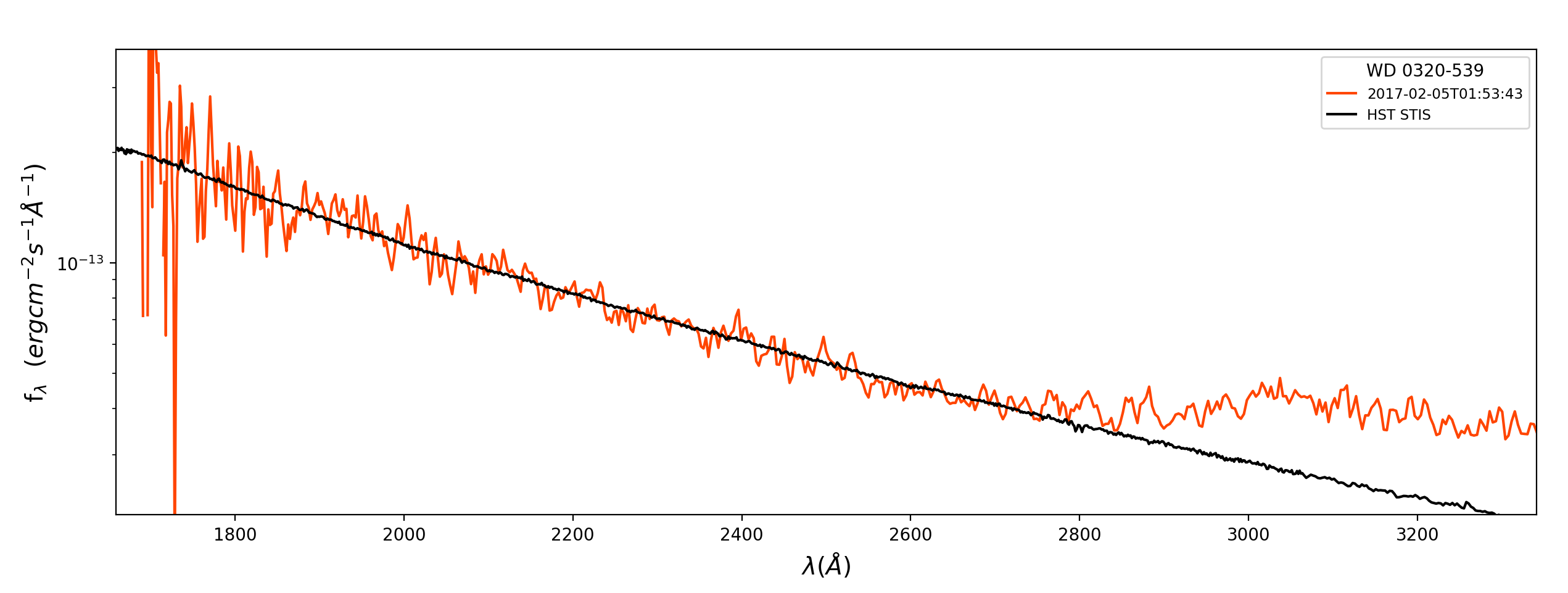
Figure 4 shows UVOT spectrum of the 14th magnitude calibration white dwarf “WD0320-539” compared with an HST spectrum. For this hot source, the second-order UV light is already present at 2850 Å, as seen in the excess flux compared to the HST spectrum.
More examples using the new calibration are (also linked from grism):