UCL MSSL Swift USA Swift UK Grism Home
NOTE: The following describes the accuracy of anchor and wavelength for
observations of the Grism+lenticular filter combination only.
Verification method
The wavelength calibration was verified using the new calibration file, and the calibration spectra. Of course, using the same spectra for deriving the calibration and verifying them is no more than a check that the wavelength calibration is internally consistent, but the number of free parameters in creating the wavelength calibration is kept to a minimum by using a simple scale factor to scale the Zemax model dispersion. The scale factor was allowed to vary over the detector as modeled by a smoothing bispline to fit the calibration observations.How to find the spectra and wavelength accuracy plots of the wavelength calibration sources
There are for each of the 29 calibration observations figures showing the spectrum both as a function of wavelength and pixel position. These were not flux calibrated, so they are in the observed counts. They have not been shifted to adjust for shifts in anchor position, nor corrected any other way, since they serve to show the result of applying the wavelength calibration and anchor position determination to each spectrum. The estimated error has been derived from these spectra by determining the mismatch between the extracted spectrum and a reference spectrum. In order to make the data accessible and organise the data according to their anchor position on the detector, two clickable maps are provided on this page where clicking on the anchor position opens a page with the spectrum or accuracy plot.
A clickable map for count rate spectra
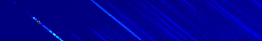
Here the count rate calibration spectra can be found. The top panel as a function of fitted wavelength, the bottom panel as function of pixel coordinate. The stronger lines have been identified and a vertical line has been plotted at the correct wavelengths. Any shifts between the predicted line position and the actual spectrum can be seen in the top panel as an offset.
The count rate in the spectra can be seen to vary across the detector, which is partly due to variations in sensitivity, and perhaps also to variablility in the source, which was chosen for calibrating the wavelengths using the many spectral lines. Details can be found in the flux calibration elsewhere.
The calibration file used was swwavcal20090406_v1_mssl_ug200.fits. In some browsers the maps do not work. In that case the plots/images can be found here.
How to read the wavelength accuracy plots
Wavelength accuracy plots were made for each useful calibration spectrum. The format of the accuracy plots is to have two panels.Upper panel: Since the main variation of the dispersion can be represented by a constant with a linear term, those have been divided out in the top panel of the accuracy plot. The higher order terms are zero at the adopted anchor points for a perfect anchor position, which for the UV-clocked grism mode is ~2600 Å. The figures also show the dispersion from the scaled Zemax optical model for the appropriate position, as interpolated by a polynomial. After extracting the spectrum with the new calibration file, and measuring the line positions, the measured line positions have been plotted as blue dots.
The lower panel of these wavelength accuracy plots shows the remainder after subtraction of the predicted position. The measured position was found as a the pixel distance to the anchor point by applying the inverse dispersion relation, while the predicted position shows the correct wavelength. If the model dispersion is good, the difference can be divided into an offset and a random looking spread around that offset. The values for the offset and the standard deviation from the spread are given in the plot. In some points near the edges of the detector, the scaled model dispersion deviates and the points will not evenly be distributed around some mean offset.
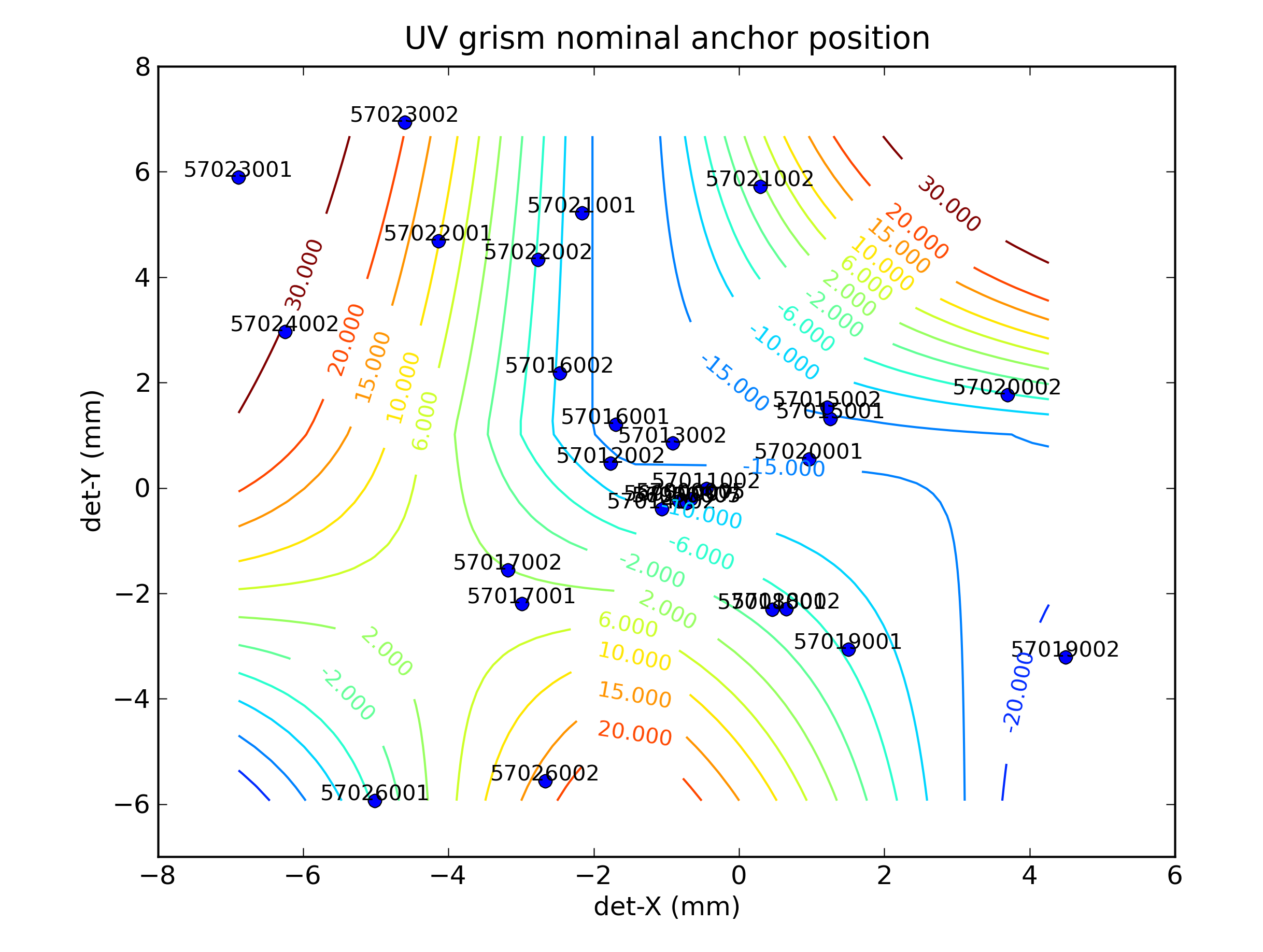
A clickable map for wavelength accuracy plots
The map below provides links to the wavelength accuracy plots.It should be noted that the contours can be a bit misleading. Take for example the 57021002 observation in the top right corner. While the contours indicate a wavelength scale offset of +2 A, the actual value is -12.4 A. The reason is that there is an additional uncertainty in the position of the anchor point as determined here from the aspect solution based on observations in a lenticular filter. That uncertainty is thought to be largely due to a possible drift of the pointing during the observation which can typically be around 4 pixels, which for a dispersion of 3.2A/pixel translates to about 13A.
Although an attempt has been made
to provide accurate and useful data, there is no absolute guarantee
that these are perfect or the latest version available. Eventually,
much of the newer developments will appear the the Swift UVOT support
site at HEASARC.
design by Paul Kuin (©2010)
