Several parameters determine the RGS effective area. The first is the effective area of the mirror modules (see § 3.2.2). Next, the amount of light from the mirrors intercepted by the grating arrays is a key quantity and how much of this light is diffracted to the different spectral orders and then absorbed on the RFCs.
The next factor influencing the RGS photon efficiency is the RFC CCDs' quantum efficiency (QE). This varies from 70% to 95% over the RGS passband from 0.35 to 2.5 keV. The value of 70% for the lowest energies will drop (by up to about 10%) when event selection with a lowest photon energy threshold is performed. The QE, without energy threshold selection, has been taken into account in the calculations of the effective area of the RGS, as displayed in Fig. 54.
To assess the total efficiency of the RGS instrument per spectral order, the efficiency with which the different spectral orders can be selected must also be taken into account. One can see in Fig. 47 that the RGAs' spectral orders spatially overlap in the dispersion direction. However, the intrinsic energy resolution of the CCDs allows the separation of X-ray photons in different orders, i.e., photons which are of different energies, but have the same position along the dispersion direction. Default masks for the spatial extraction of photons from the different orders (using PHA vs. dispersion coordinate plots, as in Fig. 47), are provided as part of the Current Calibration File (CCF) for each XMM RGS instrument. The expected efficiency in the post-observation RGS order selection with the SAS is ca. 90%. Since the order selection is part of the offline processing, it is not included in the effective area calculations presented here.
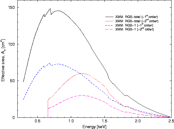 |
Fig. 54 displays the effective area of both RGS units together, taking into account the factors listed above. This is ca. 150 cm2 at 1 keV. Seam losses between the CCDs were excluded from this calculation.