
GRB 130427A Swift UVOT uv grism spectrum: the deconvolution of smearing from attitude loss
Creation of the kernel of blurring motion
In order to do a deconvolution of the blurred image, the motion of the source over the detector during the exposure must be found. To do that, we use the zeroth order of the GRB spectrum and a zeroth order of a good observation.
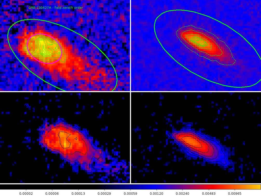
Figure 1. The top row are the zeroth order images of GRB130427A (left) and a zeroth order in the image of obsid 00055200001[2] (COM). The bottom row shows the images after background subtraction and normalisation.
A region of 80x60 pixels in the detector image has been selected, centered approximately on the peak zeroth order emission. The centers were at
GRB:  00554620992ugu_dt.img  gu388741990I  [983, 847]
COM:  00055200001ugu_dt.img  gu132535224I  [1394,864]
The background image was made in two steps:
bkg = GRB
bkg[ GRB > (GRB.mean()+GRB.std()] = GRB.mean()
bkg[ bkg > (bkg.mean()+bkg.std()] = bkg.mean()
replacing the values higher than the mean plus one standard deviation with the mean. The same was done for the COM images. The background was subtracted and the resulting image normalised to the counts in the area visibly above the background as follows:
GRB = GRB - bkg
GRB = GRB/(GRB[25:78,2:41].sum())
COM = COM - combkg
COM = COM/(COM[20:63,13:41].sum())
The zeroth order images were saved in fits files:
filter/normalisedGRBzerothOrder.fits
filter/normalisedGoodzerothOrder.fits
To obtain the kernel for the blurring, the GRB zeroth order image needs to be deconvolved with the good image of the COM zeroth order. To do that I am using the “LUCY” program from the “STARLINK” software. Since this takes special formatted input files, the fits files need to be converted first using the “FITS2NDF” program.
The “STARLINK” was grabbed from the GIT repository, built and installed.
The files were converted to the “STARLINK” NDF format using:
convert

cp normalisedGRBzerothOrder.fits infile
fits2ndf infile outfile fmtcnv=T
mv outfile.sdf grb.sdf

cp normalisedGoodzerothOrder.fits infile
fits2ndf infile outfile fmtcnv=T
mv outfile.sdf good.sdf

kappa
lucy  grb.sdf good.sdf first aim=0.0001 niter=60
ndf2fits first.sdf first.fit
lucy grb.sdf good.sdf second aim=0.0001 niter=60 start=first.sdf
ndf2fits second.sdf second.fit
Then the first result was used to make an image and the second to build a contour map. The statistics were compared using the “stats” command and showed sufficient convergence.
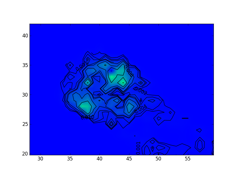
Figure 2. The resulting filter after applying the Richardson-Lucy method.
The distance between the main peaks as slightly over 7 pixels. Presumably this shows the positions that the spectrum was at over time. Obviously this would mean that the observation was taken whilst in mainly two locations. The orientation of the motion between these locations is consistent with that found from the analysis of the motion in the event data. The direction of the motion is mainly across the dispersion direction,
Correcting the grism image
Finally, the grism observation was read into Python, and the image was written to a new fits file (primary), grism.fits, followed by a conversion to NDF:
[paul-mssl2l:uvot/image/filter] kuin% fstruct grism.fits
No. Type     EXTNAME      BITPIX Dimensions(columns)      PCOUNT  GCOUNT

 0  PRIMARY                -32     1987 2046                   0    1
[paul-mssl2l:uvot/image/filter] kuin% fits2ndf grism.fits grismndf fmtcnv=T
Finally, the image was processed with the filter, and converted to fits:
lucy grismndf.sdf second.sdf newgrism aim=0.1 niter=5

PSF area is about 27 by 20 pixels.

X-axis margin is 27 pixels wide.
Y-axis margin is 20 lines wide.
Internal file size is 2041 by 2086.

Using a constant noise value of 0.329904.
Initial normalised chi squared is 0.572227

Iteration 1
  Normalised chi squared: 0.296033


Iteration 5
  Normalised chi squared: 0.252322


[paul-mssl2l:uvot/image/filter] kuin% ndf2fits newgrism.sdf newgrism.fits
The new fits observation was read into Python, as well as the grism observation, ‘sw00554620992ugu_dt.img’. Then, in the new data array values less or equal to zero were set to 1e-3. Finally, the array was copied in place of the old one, and a new fits file was written. That file was subsequently renamed to the old name for further processing. The image was inspected using DS9 and looks much sharper.
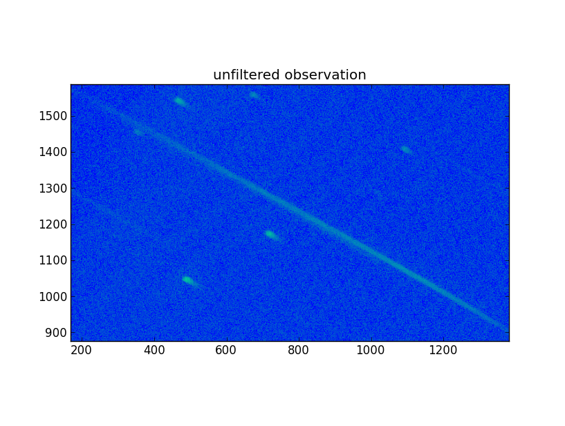
Figure 3. The unfiltered image (section).
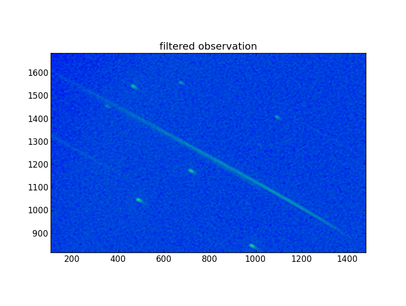
Figure 4. The filtered image (section).
The spectrum was extracted using the white filter images extracted from the event data for positioning. The spectrum may still be off by some pixels due to the movement of the satellite. Probably the kernel adjusted to some mean over the 50 second period, but we should allow for about 7 pixels just for that.
A better spectrum
The white event data had been processed into a file with many individual extensions, each aspect corrected. This file, sw00554620992uwh_sk.img was copied into the directory, after which the default program was run as
uvotgetspec.getSpec(ra,dec,obsid,1,clobber=True)
The calibrated anchor offset, as derived using the last white image extension (22), from the spectrum was 6 pix.
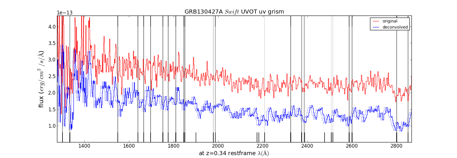
Figure 5. Comparison of the unfiltered tot the deconvolved spectrum. An idea of the uncertainty in wavelength scale can be gotten because the deconvolved spectrum was plotted with a 15A offset also.
The
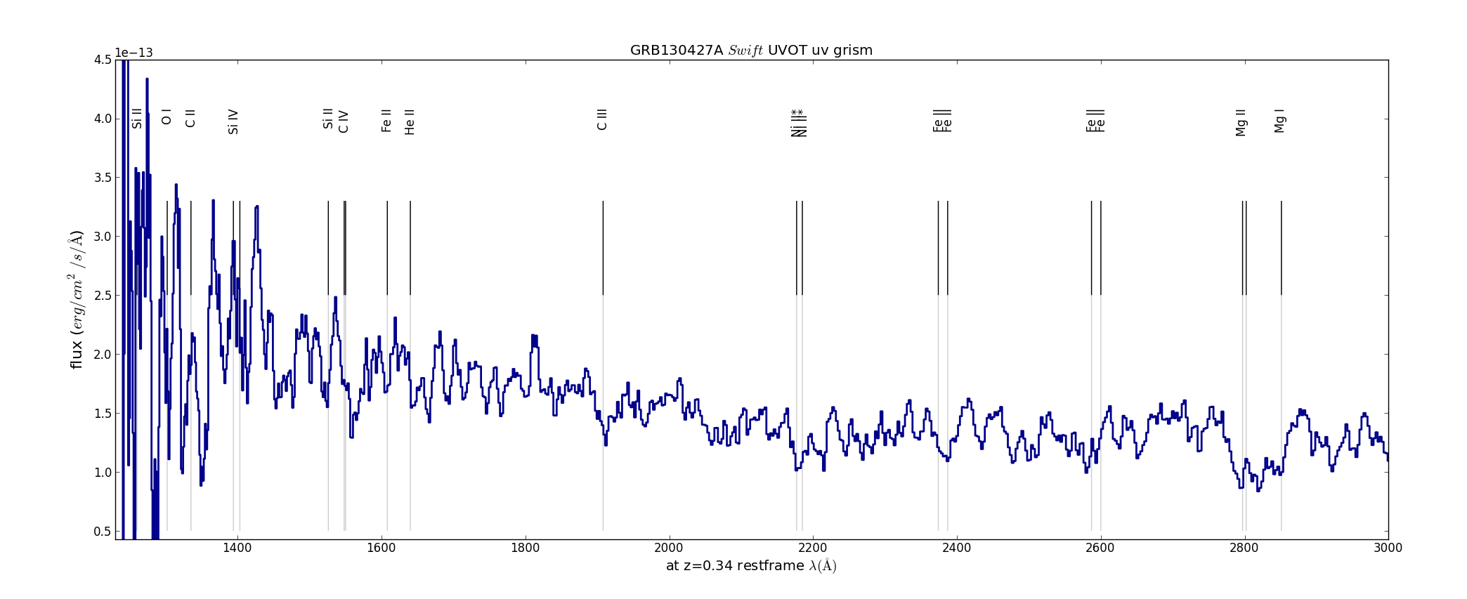
Figure 6. The deconvolved spectrum with line identifications.
Spectral line identifications:
| wave | identification @z=0.34 |
|---|---|
| 1260 | Si II 2P - 2D ? |
| 1262 | C I 3P - 3P |
| 1277 | C I 3P - 3D |
| 1280 | C I 3P - 3P |
| 1302 | O I 3P - 3S |
| 1305 | O I 3P - 3S |
| 1330 | C I 3P - 3P |
| 1335 | C II 2P - 2D |
| 1368 | Al I 2P - 2S |
| 1394 | Si IV 2S - 2P |
| 1402 | Si IV 2S - 2P |
| 1450 | unid |
| 1526 | Si II 2P - 2S |
| 1548 | C IV 2S - 2P |
| 1551 | C IV 2S - 2P |
| 1640 | He II |
| 1660 | C I 3P - 3P |
| 1908 | C III 1S - 3P |
| 1964 | unid |
| 2139 | N II 3P - 5S |
| 2143 | N II 3P - 5S |
| 2177 | Ni II* 4F - 4F |
| 2185 | Ni II* 4F - 4F |
| 2206 | Si III ? |
| 2334 | Fe II a6D - z6P uv3 |
| 2344 | Fe II a6D - z6P uv3 |
| 2349 | Fe II a6D - z6P uv3 |
| 2374 | Fe II a6D - z6F uv2 |
| 2383 | Fe II a6D - z6F uv2 |
| 2387 | Fe II a6D - z6F uv2 |
| 2389 | Fe II a6D - z6F uv2 |
| 2396 | Fe II a6D - z6F uv2 |
| 2405 | Fe II a6D - z6F uv2 |
| 2505 | unid C II 2512? |
| 2587 | Fe II a6D - z6D uv1 |
| 2600 | Fe II a6D - z6D uv1 |
| 2632 | Fe II a6D - z6D uv1 |
| 2715 | Fe II a4D - z4D uv63 |
| 2740 | Fe II a4D - z4D uv63 |
| 2748 | Fe II a4D - z4D uv63 |
| 2770 | Fe II a4D - z4D uv63 |
| 2796 | Mg II 2S - 2P |
| 2803 | Mg II 2S - 2P |
| 2832 | unid |
| 2852 | Mg I 1S - 1P |
| 2929 | Mg II 2P - 2S |
The dispersion errors are not random, but increase towards the short and the long wavelengths, being fixed at 2600A. Checking the calibration spectra (WR86 00057020001[1] was taken with her anchor within ~20pixels on the detector of that of the GRB spectrum, and the WR52 spectrum taken at the nearby boresight) with the wavelenghts from the calibration shows that the assigned wavelength scale is ~14A too short at 1700A, and ~25A too short at 5800A, but there is no clear offset in the 2200A-3300A region. This is perhaps due to the adoption of a single scale factor to the zemax model dispersion.
The CIV and SiIV absorptin lines appear both blue shifted by about 10A in the rest frame, which would imply a velocity of ~2500km/s relative to the lines from the neutral and singly ionised spectra lines.