
General comments about the flux calibration
The old web pages are here:
Introduction
The post launch calibration of the Swift UVOT instrument included a calibration for the grisms for sources placed in the centre of the field of view. We usually refer to this as the default position. Here the first order spectrum fall over the middle of the detector image, and the zeroth order is offset to the lower right hand corner.
Over time it was found that the source was not always placed in the centre of the field of view unless a special procedure was used to refine the pointing. Spectra were taken that appeared at various positions over the detector for more than a year, without much control. It was found that the dispersion solution was different for those offset positions. Also, when it became clear that orders partly separated in spectra placed in the upper right corner in the UV grism, the flux calibration needed to be updated.
Until early 2012 calibration spectra taken at offset positions seemed to show that there was not much variation of the sensitivity over the face of the detector. Those studies were rather short ones, and indicated that the flux calibration should be good to about 20% or better. The early calibration did not take into account the coincidence loss which was only studied for point sources at that time.
The second order in the uv grism is bright at the blue end of the order it can carry close to 70% and falling of the flux compared to the first order for a certain wavelength. Of course the second order seems fainter due to lower dispersion and broader PSF while it is offset along the first order. In the v grism, the second order is relatively fainter, though we don’t know quantitatively by how much, and is displaced further along the spectrum.
Although there is order overlap of first, second and third order in both grisms, there is a big difference depending on the colour of the source. Whereas for a very blue source the second order starts affecting the flux above 2700A, for a redder source with an F0 spectrum the order overlap did not become an issue until about 4900A. So the intial flux calibration was extended using some redder calibration sources up to 4900A.
It had been recognized rather early on that the issue of coincidence loss in the grism, the varying order overlap, the curvature of the spectral extraction in the UV grism, and the sensitivity variation over the detector needed further study and better tools for spectral extraction. The new spectral extraction code written in Python allows us to address these issues now and improve the flux calibration. Our goal is to get an effective area accuracy to within 5% for the weaker sources with low backgrounds and to within 20% for brighter ones with coincidence loss by correcting for it. In the uvot grisms the background itself can suffer from 1-10% coincidence loss already, since a wide wavelength band passes through.
The calibration overview
The following approach was taken to ensure a consistent and transparent way for the flux calibration.
- Flux calibration sources were selected from the CALSPEC collection which are thought to be accurate to within 3%
- calibration sources include uv-bright DA White Dwarfs, F subdwarfs, F0 main sequence, and TBD sources in order to cover the first order wavelength in parts with negligible second order contamination
- A Zemax optical model calculation was done in order to identify the overall sensitivity variation over the detector
- The calibration sources were observed at the centre of the detector, both very weak, moderately brighter, and bright
- the spectra with low backgrounds were selected in order to reduce the effect of coincidence loss
- the coincidence loss was corrected using the established correction developed for uvot photometry
- bad areas in the individual spectra were flagged and not used
- spectra were shifted to correct for the errors in wavelength
- for each spectrum the effective area was computed, keeping track of errors, and coincidence loss
- effective areas were summed, weighted according to the errors
- missed problems were flagged and corrected, after which we reprocessed
- additional smoothing of the effective area was done depending on the quality, differs by wavelength region
- the new effective area was used to plot the calibration spectra used with the CALSPEC spectrum
- the effective areas were computed first for the default positions near the centre
- the coincidence loss correction to the spectrum was adjusted (X)
- a final rerun with the better coi-correction was made to derive the effective areas (X)
- effective areas at offset positions were determined (X)
- the Zemax model sensitivities were lined up with the observed effective area (X)
- the model sensitivities and measured effective were combined for the overall product (X)
- “(X)” means that work is in progress
Effective Area
The input to the calibration are trusted flux calibrated spectra of selected calibration sources, the uvot observations of those sources, and the output is an effective area which gives as function of wavelength the scaling from photon rates to flux. ; The relation is as follows:
EA = Eph . CR / F
Where the effective area EA is in units of cm2, Eph the photon energy in ergs, CR the count rate per 1A wide spectral bin, and F the flux of the trusted calibration spectrum in units of erg /cm2/s/A. For each grism mode the details, including the calibration sources used are listed on their separate pages which can be selected from the menu.
Nearly all calibration sources are taken from the CALSPEC library. The CALSPEC spectra were used to compute synthetic uvot photometry which was compared to available observations (GSPC P177D, GSPC P-041C). The photometry is consistent within the uvot zeropoint errors. In part that is to be expected since some of the sources were also used for the uvot photometric calibration.
Coincidence loss
As in other photon counting detectors, counts are lost at high count rates. For the UVOT the coincidence-loss (sometimes called pile-up) has been well studied for the photometric calibration of point sources. Also, coincidence loss in the background was studied in Breeveld et al. (2010). They found that for extremely high backgrounds the coincidence loss in the background only (diverged from that of a point source. A simple first order polynomial correction to the coincidence loss gives a better fit.
We work from the rotated spectrum, where essentially the spectrum varies with wavelength along the x-axis, while we integrate across the spectrum along the y-axis in bins, one pixel wide in x. One x-bin covers a variable amount of wavelength depending on the dispersion relation. The count rate in the spectrum is determined by measuring the counts in a slit of certain width, dividing by the exposure time, and doing an aperture correction for the counts that fall outside the extraction slit.
For clarity, the effect of the coincidence loss is parametrized as a coi-factor which I defined as:
Background:
coi_bkg_factor = incident_bkg_count_rate / observed_bkg_count_rate
Net Spectrum:
coi_net_factor = incident_net_count_rate / observed_net_count_rate,
where:
incident_net_count_rate  = (incident_total_count_rate - incident_bkg_count_rate), and
observed_net_count_rate = (observed_total_count_rate - observed_bkg_count_rate)
The background is taken for the same number of pixels as the spectrum. The spectrum measurement includes the background and yields ; the incident_total_count_rate.
The coincidence loss factor, defined as the incident count rate by the measured count rate, in the background of the calibration sources is typically about 1.02 to 1.04, though values as high as 1.08 are seen in some images. Of course we can not measure the incident count rate, but employ the following method:
For the background:
- multiply the background count rate per 1x1 pixel with 315 which is the
number of 1x1 pixels in a 5.02” aperture used in the photometry, lets call that CR.
multiply CR with the frame time tf to get the counts per frame CPF, typically CPF ~ 1.
correct with the point-source formula:
CFc = -ln(1.-CPF)/alpha
alpha is the dead time correction; “ln” the natural logarithm.
multiplying CPF by the polynomial for counts lost due to centroiding, etc.
CPF’ = (1 - 0.67 * CPF) .
recompute CFc using CPF’
the coi-factor for the background is then CFc/CF which is identical to that for UVOT photometry.
For the spectrum:
- boxcar smooth the extracted count rate spectrum with known width over 26 pixels in the dispersion direction
- divide the net count rate over the width of the extraction, and multiply by 315
- perform the aspect correction to the net count rate and multiply with the frametime
- add in the background CPF to get the total CPF
- compute the initial CFc for the total CPF
- correct the net CPF using a polynomial in CFc.
- recompute CFc for the total count rate
The approach recognises that the spectrum coincidence loss is in addition to that of the background, but with different scaling since the profile is extended in one dimension, not flat. In the limit the background rate is recovered. The polynomial for the net CFc is determined by calibration of the flux of sources of varying brightness. A good first approximation is a constant.
Using the coi-factors, it is relatively straightforward to correct the observed background and net rates. Note that the background factor includes the deadtime correction of about 1.6%. The initial coi-correction gives a fit to the flux that is good to within about 25% for all spectra, and is within 10% for the fainter spectra.
Examples of the coi-correction
In the following figures, the current success of the new approach can be judged. Some spectra show contamination by zeroth orders of background stars - the peaky things. If many calibration spectra were taken with the same spacecraft roll angle, they all show the same contamination.
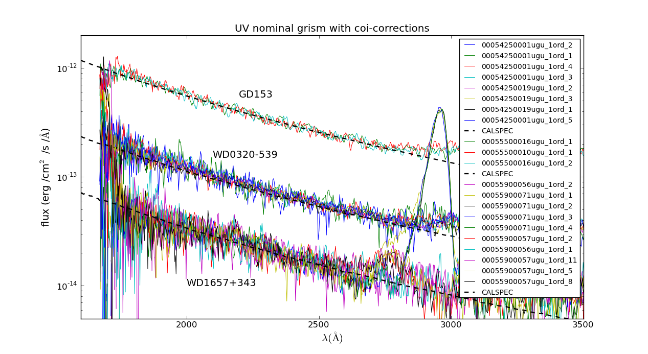
Flux calibration uv grism nominal mode. Comparison of WDs with range in brightness for initial coi-correction (first cut 2012-09-26)
Above about 2740A, the second order overlap begins. The second order uv response in the uvot uv grism is strong, from 50-100% of the first order in flux,
And for the redder sources:
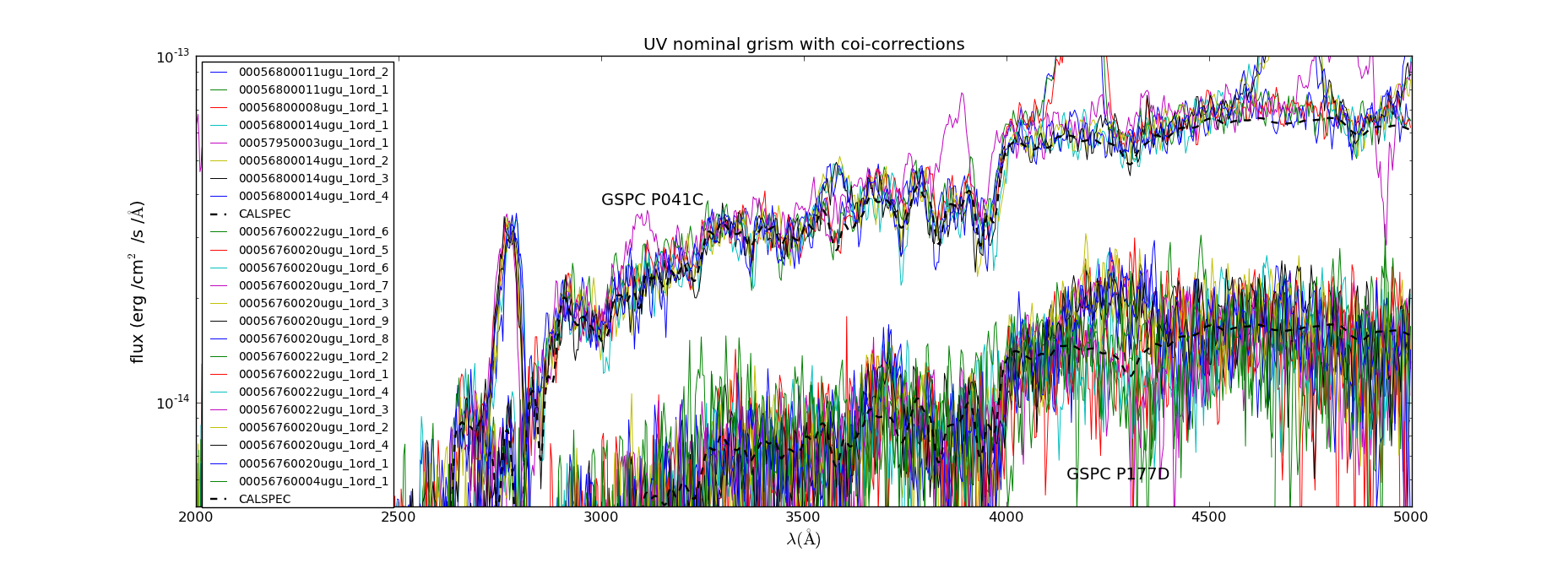
Flux calibration uv grism nominal mode. Comparison of cooler star spectra with range in brightness for the (2012-09-26) initial coi-correction (2012-09-26).
And similar for the clocked grism:
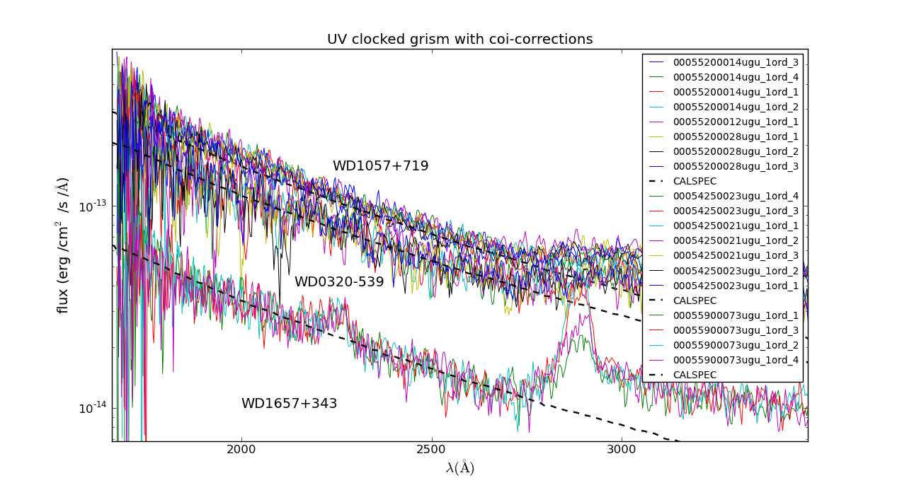
Flux calibration uv grism clocked mode. Comparison of WD spectra with range in brightness for the initial coi-correction.

uv grism clocked mode. Comparision flux after initial form of coi-correction for F0V star spectra with range in brightness.
The effective areas that were used for the flux calibration of these spectra were based on the calibration data with the lowest backgrounds with extraction widths of 2.5 sigma halfwidth.See the pages for the various modes [nominal, clocked] for more details.
The faintest source, the GSPC P177D star of spectral type F0V, the coi-factor on the net count rate (after coi-corrected background subtraction) at 3000A is 1.05. That is completely dominated by the background since the coi-factor for the net rate is about twice that in the background in the limit of a spectral flux small compared to the background which is due to the logarithmic nature of the coi-correction. The slightly brighter sources are still dominated by the background as the typical coi-factors at 3000A show.
Typical coi-factors uv grism
| Source | Coi-Factor net spectrum | Coi-Factor background |
|---|---|---|
| WD1057+719 | 1.086 | 1.05 |
| WD0320-539 | 1.084 | 1.04 |
| GSPC P177-D | 1.050 | 1.02 |
| GSPC P041-C | 1.067 | 1.03 |
| G63-26 | 1.10 | 1.03 |
Images with backgrounds which were exceptionally high (background coi factors >1.06) were not used. This also illustrates that not correcting for the background induced coi-loss causes flux errors in the order of 5% already.
The grism images were reduced using the ` “uvotpy” solftware <../uvotpy/UVOT_grism_python_software.html>`_. The images were compared to DSS images by blinking in “DS9” to identify faint sources not automatically detected in uvotpy. The spectral regions affected were flagged in a database of calibration observations. The individual spectra were then used to derive effective areas whilst keeping track of the measurement error, quality flags, and coi-factor. Finally the effective areas were summed using the errors to weight the various values, selected by source and position on the detector. At that point the coi-factors were applied. The error based on the spread in the individual effective areas was also determined, and usually exceeds that in each measurement. Any problems found were corrected and the analysis redone. Finally, a merged effective area from all the sources was derived, and its error.
Shape of the effective area and the difference between that in the nominal and clocked modes
The shape of the effective area is to a large extent determined by the physical properties of the lenses and prisms/grating used in the grism assembly. So we would expect some variation in overall sensitivity over the face of the detector, but the overall shape of the effective area to be pretty much the same. Since the clocked mode is just the same grism, but offset with respect to the instrument boresight, it is not surprising that the effective areas as derived from the two modes are nearly the same.
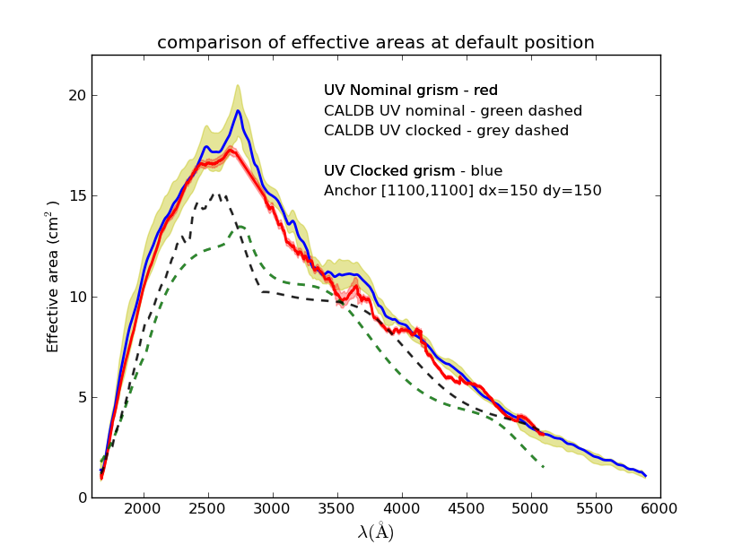
Old and new effective area of UV grism - both modes
This figure shows the independently derived first cut-effective areas for the clocked and nominal grism modes. The 1-sigma RMS errors [based on the deviations from the individual contributions to the mean] have been indicated as shaded areas. The old effective areas, which are smaller since no correction was made for coincidence loss and deadtime, are shown for comparison. The difference below 2000A is partly due to the introduction of a curved extraction slit. Above 4900A a larger error has been created ad-hoc to show higher order contamination.
The wiggles at longer wavelengths [3000-5000A] in the new effective area curves are mostly due to weak, unresolved, background sources in the calibration spectra. The similarity in the effective area curves for nominal and clocked grism modes is obvious.
Modeling the flux by detector position
A further verification was made by computing Zemax optical models for the flux normalized to that at the model boresight position. This is particularly useful in the clocked modes, where the reduced aperture affects the throughput. The models confirm the overall variation in measured spectral flux that we observe. Work on the model comparison and possible integration in the flux calibration is continuing.
The errors in the flux
Theoretically, the errors in the flux should be dominated by Poisson counting statistic, with some modification from the coincidence loss. The errors were derived this way, and flowed down in the effective area analysis for each individual spectrum that was processed into an effective area. However, we use many spectra and so can derive another error estimate on the effective area from the deviations from the average of all those spectra. That average is typically about 3 times larger than the errors flowed down from the counting statistics. Clearly another source of error dominates. Without going into much detail at this point on the source of that error, practically speaking that means that the effective error in the flux is larger than that derived using counting statistics, i.e., the error in the output file should be multiplied by a factor of about 3.
This deserves a more careful study, and at some future time this will be done. For now, use the error estimates with the above remarks in mind.