Swift UVOT UV-clocked grism second order calibration

overview

The UVOT Clocked Grism mode second order is usually fainter than the first order. However, for very brigh object, when observed in either the upper right hand corner, or in the lower left hand corner, one can observe the UV part of the second, third and, at times, fourth order as a bright streak separated from the main first order spectrum. The reason for the separation is that the spectrum has curvature that varies in magnitude and direction across the detector.

Curvature of the orders

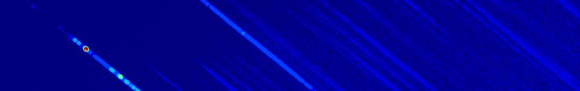
The lay of the orders for a spectrum in the upper right hand side corner of the detector is shown in the image below.

For each order a different color was used: zeroth:yellow, black:first, second:blue, third:red. 
The locations are based on the measured positions.

The curvature of the spectral orders was measured in about 30 spectra, mainly of the Wolf-Rayet star WR52, which is bright enough to show the spectral lines in the higher orders. The curvature was measureded from the rotated spectrum with reference to the anchor point in first order.  The measured curves were approximated with polynomials, third order polynomials for the first order, a second order polynomial for the second order and a first order polynomial for the third and zeroth orders. The polynomial coefficients were then each fitted with a bilinear or bicubic polynomial with reference to the first order anchor point on the detector.

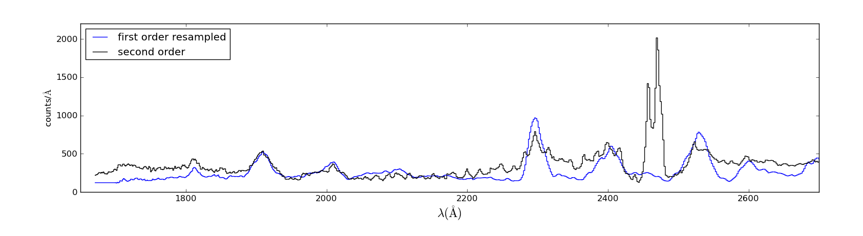
Second order flux as compared to the first order flux

For the first estimate we are using the following spectrum (1st order anchor point [1468,1590] on detector):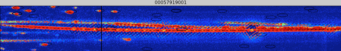



The black vertical line in the image indicates the location of the anchor where it crosses the spectrum. Circles indicate where zeroth orders are found in USNO-B1 with a B2 magnitude larger then some limit.  There are no zeroth orders on the rhs in the clocked image. The tail end of two other spectra can be seen to enter the image from the left. The dashed lines are the curved slit centres from the calibration of the curvature of the orders. 


A rough estimate of the second order sensitivity can be obtained by extracting the data from the image shown above which is located in the upper right hand quadrant of the detector where the second order separates from the first order.

The plot above was made by extracting the first order and second order counts using a fixed curved slit. The counts per bin were converted using counts/Å using the dispersion relations. Since the interpolated dispersion relation for the second order was not accurate enough, it was rederived for this spectrum. Prior to deriving the ratio plot below, the first order flux/Å was resampled to match the second order points. (Without it, the current second order dispersion accuracy is not good enough that the line positions in first and second order match this good. Even with perfect second order dispersion, inaccuracies in the anchor position will mess up the matching to some degree.)



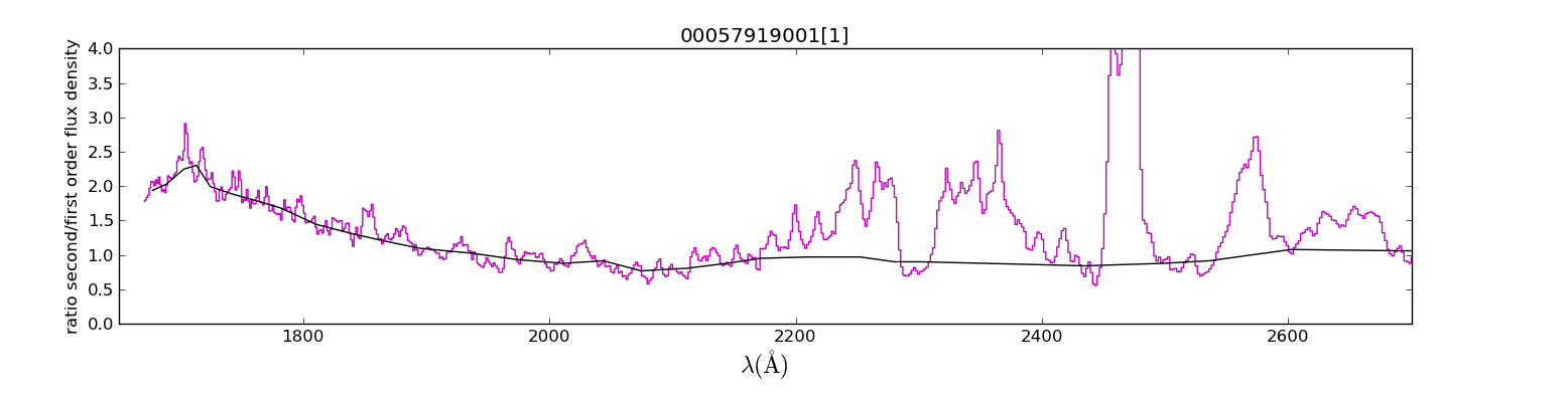
The ratio R21 of the second order flux/Å  over the first order flux/Å. The relation above 2100Å diverges from the expected ratio of flux densities, since the second order starts picking up the wings of the first order flux. Also, in the stronger lines, the first order suffers from coincidence loss, which accounts for the bumps, except for the strong peak around 2460Å which is due to the very extended wings of the first order 4649Å line being picked up in the second order.

The ratio here is larger than seen in the ground calibration for the nominal mode at the centre of the detector, and suggest that perhaps the ratio continues to decline past 2100Å. So this result must be used with caution for the longer wavelengths.