Swift UVOT UV-grism flux calibration for the nominal mode

Flux calibration of the first order

The method for deriving the effective area can be found here. A detailed discussion of the coincidence loss will be added later. Below the details for the nominal uv grism are discussed, including the sensitivity variation over the detector. 

The assumed sensitivity loss for the calibration was taken to be 1% per year, which is consistent with the sensitivity loss seen in the majority of the lenticular filters.  The major source for sensitivity loss is thought to be the Multi Channel plate Photomutiplier, which would affect the throughput of all filters equally.

The sources were chosen to be as unaffected by coincidence loss of the detector as possible. Typically, the background in the grism image suffers from 2-5 % (in exeptional cases up to 10%) coincidence loss.   Coincidence loss in the background has been studied and the effectiveness of the standard correction in that case was discussed in Breeveld et al. 2010.  The backgrounds are all low enough to assume this correction. The same correction was also applied to the total of the spectrum plus background scaled to include 315 (1x1) (sub-)pixels, i.e. the same area on the detector as used for point sources and the background.   For the weak spectra that we used (with the normalised count rate not much above the background), this is considered a good first order correction. 

The second order flux calibration has been planned for future work.

Effective area for the default position

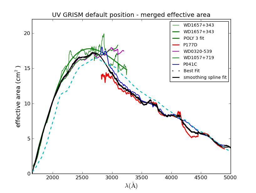
The figure contains the averaged effective area curves which were derived for several sources. Each source was observed repeatedly. The figure only shows the averaged curves. The weakest spectra show the largest noise. Details can be found in the table below. The WD1657+343 spectrum between 2100 and 3200A was fitted with a 3rd order polynomial before averaging with the other two WDs. The data between 2750 and 2940 are so noisy, that they were not used for the final fit. The best fit was derived from the averages from the different sources at each wavelength, weighted based on their error.  Finally, a smoothing spline was fitted to those averaged values. Above 1700A the error is within 5%, below 1700A less than 10%.  A correction for the coincidence loss  was made to all data.  The differences between the weakest and slightly brighter stars are not significant.  The higher uv effective area in the new calibration as compared to the old one may be due to a better account of the curvature of the spectra at low wavelengths.

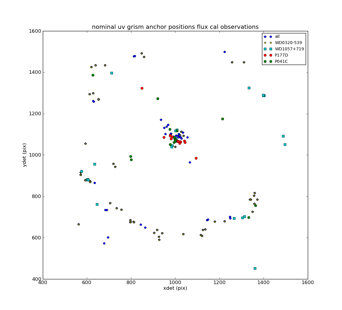
Available Calibration Spectra

The position of the anchor points of selected calibration sources has been plotted to show the coverage of the detector.  The spectra extend further over the detector, and therefore most observations will fall within the region shown.

The following calibration sources were used:

Calibration source	RA	Dec	V mag	Spectral type and kind	source reference spectrum	useful wavelength range for calibration
WD1657+343	16:58:51.12	+34:18:53.3	16.4	DA White Dwarf	CALSPEC	1600-2800 (3400)
WD0320-539	03:22:14.83	-53:45:16.4	14.9	DA White Dwarf	CALSPEC	1600-2800 (3400)
WD1057+719	03:48:50.19	-00:58:32.0	14.68	DA White Dwarf	CALSPEC	1600-2800 (3400)
GSPC P177D	15 59 13.59	+47 36 41.8	13.48	F0 V star	CALSPEC	2900-4900 (6000)
GSPC P041C	14 51 58.19	+71 43 17.3	12.01	F0 V star	CALSPEC	2900-4900 (6000)

The useful wavelength range is limited due to the order overlap. At some locations on the detector the second order starts affecting the first order later and the extension is put in brackets. The second order overlap for the F0 V stars starts later due to the faintness of the blue spectrum.  The Johnson V magnitude for these "faint" sources is higher for the White Dwarfs, since they are so more uv-bright.

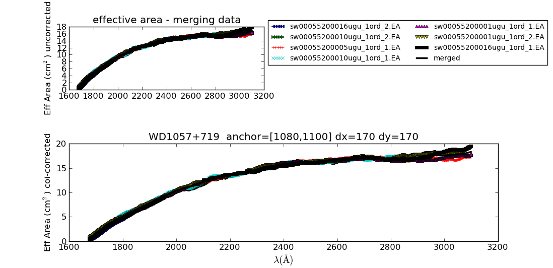
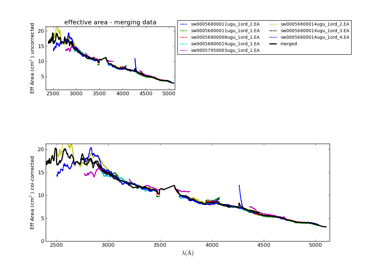
Combining the data

In order to get an idea of the consistency of the spectra for an individual source, the following figures show the data for WD1057+719 and P041C. Each figure shows two plots. One where the effective area was calculated without correcting the observed count rate for detector dead time and coincidence loss, one with the correction made.

 

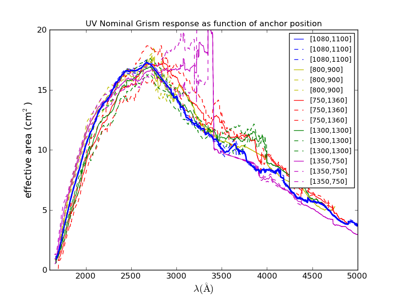
The merged effective areas at various positions on the detector

The effective area at offset positions derived from a straightforward weighted sum of the individual effective areas is shown in the figure below. The dashed curves are the (1-sigma) error bounds.  Notice that the magenta curve diverges between 2700-3400 and has also gaps due to limited amount of data. The red curve, at the top left corner is the only curve showing some perhaps significant difference from the blue curve at the default position: it peaks later, has less response in the UV and more in the visual part of the spectrum. The green curve (top right hand side) seems to show the same behaviour.

The differences are easily visible in the normalized plot below. Remember that the errors are not include in the plot below, though the differences are clearly visible as a change of the whole effective areas.  A linear interpolation has been used. The bumps above 3000A are most likely due to faint background sources and only a limited number of spectra used for similar roll angles.

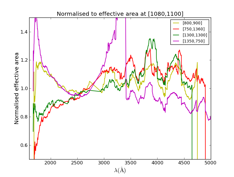
The divergence in the UV from the effective area in the centre  is considered real, while the wiggles from 2800A to the red part of the spectrum are due to noise and unresolved weak background sources. They are similar since the offset spectra for the F0V sources were taken contemporaneously.

The normalised curves can be compared to the Zemax model computations.

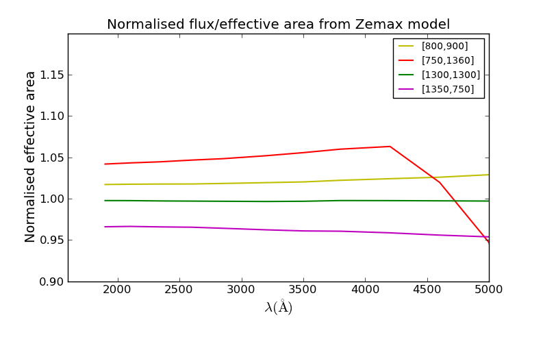
The model predicts a small variation in the normalised flux which means the same for the normalised effective areas. The drop of the red curve at long wavelengths is probably due to a misalignment of the model to the data. Below 2100A the model may not be using the exact properties of the optical materials as that data is no longer available generic properties were used.  The overall order in brightness can be seen to be similar as in the observed curves above, though the details are sufficiently different that using the effective areas from the calibration measurements should be preferable.