NOTE: The following describes the accuracy of anchor and wavelength for
observations of the Grism+lenticular filter combination only.
The visible grism dispersion is approximately 6 Angstrom per pixel, though for accurate wavelengths a third order polynomial is needed. The coefficients of that polynomial vary with the position of the spectrum on the detector, where the anchor position is used for a reference point for each spectrum.
The derivation of the coefficients was done using an early version of the uvotpy code, and were stored in the wavelength calibration file (wavecal file). This was followed by a verification of the new wavelength calibration file using the uvotpy-0.9 code, using the same set of emission line spectra of WR stars used for deriving the calibration. In 2014 a further verification was made using spectra of the sources not used in the derivation of the wavelength calibration.
The 2009 verification of the wavelength calibration
Two types of plots were made. The first type of plot
called "accuracy plot" displays for a spectrum the measured line
positions and the wavelength equation derived from retrieving the
polynomial coefficients for the appropriate position of the spectrum
from the wavecal file. The second type of plot displays the count
rate spectrum with line identifications.
The wavelength accuracy plots
Wavelength accuracy plots were made for the 28 calibration spectra. The accuracy plots have two panels. The top panel shows the wavelength as a function of the distance in pixels to the anchor. Parts of the spectrum blueward of the anchor have negative pixel coordinates and the redward parts positive pixel coordinates. The wavelengths are expressed as a third order polynomial:lambda = C0 + C1 p + C2 p^2 + C3 p^3.
The leading terms are the linear ones, so we plot
delta_lambda = lambda - lambda_linear, with lambda_linear = C0 + C1 p
This makes any discrepancies stand out much better. The plot shows the polynomial and the measured data from the line positions. (The plot also tried to show the scaled model points, but an error in the plotting program was later discovered. After correction of that error they fall right on top of the polynomial curve). The higher order terms tend to zero near the adopted anchor point, which for the Visible grism is ~4200 Å. The observed line positions from lines identified in the calibration spectrum have been plotted as blue dots.
The lower panel of the plot shows the remainder after subtraction of the predicted wavelength based on the observed position of the line. The observed position was found from the pixel distance to the anchor poin. This was subtracted from the known spectral line wavelength. The mean of the differences defines an offset that can be attributed in large part to inaccuracies in the anchor position. A random looking spread around that offset remains which is consistent with the estimated measurement error in line position of around 1 pixel.
The values for that mean and standard deviation of delta_lambda are given in the plot. In some points near the edges of the detector, the scaled model dispersion deviates and the points will not evenly be distributed around some mean offset.
A clickable map for wavelength accuracy plots
The map below provides links to the wavelength accuracy plots. Point your mouse to the desired observation to see the plot.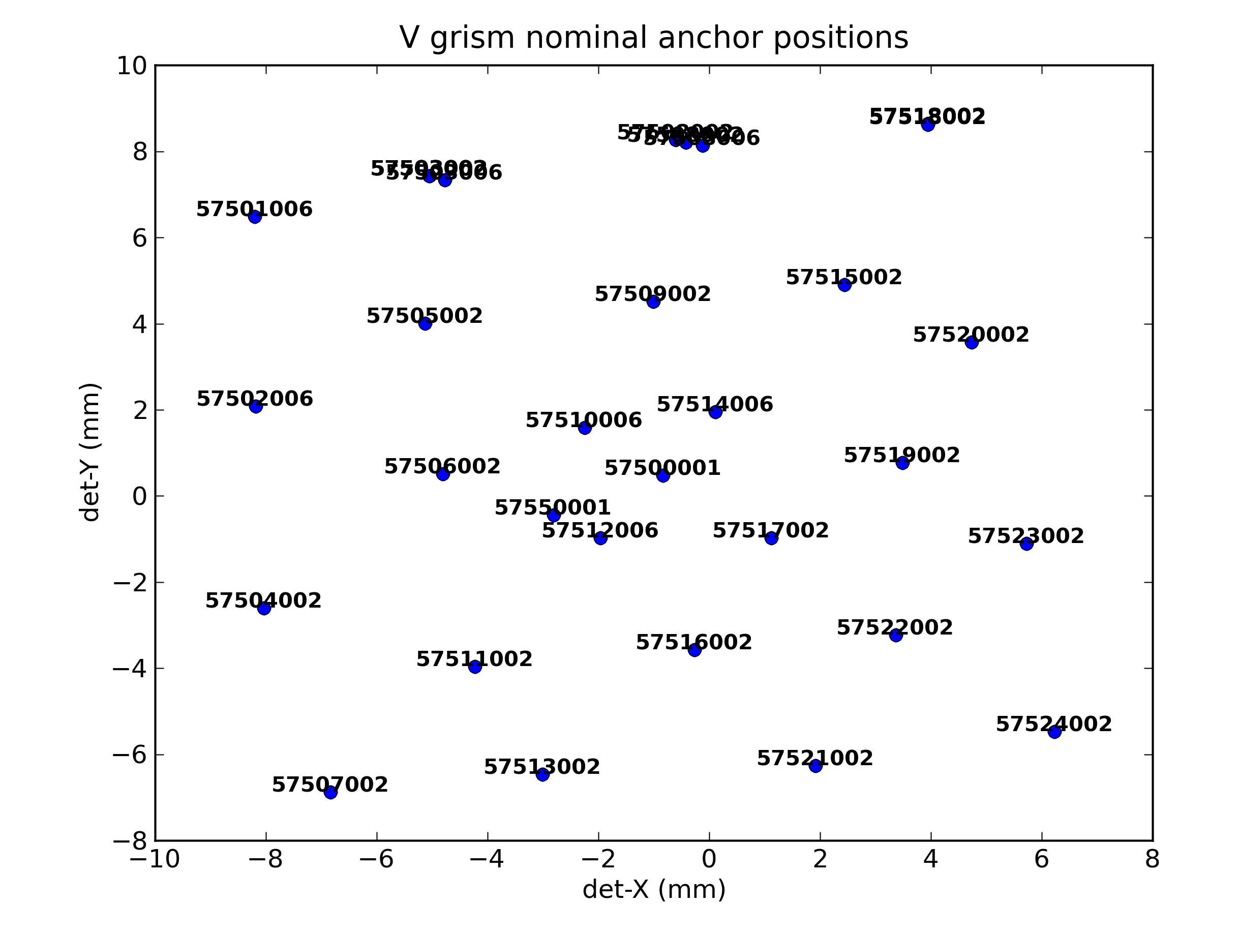
A clickable map for count rate spectra
Here the count rate calibration spectra can be found. The top panel as
a function of fitted wavelength, the bottom panel as function of pixel
coordinate. The stronger lines have been identified. Any shifts between
the predicted line position and the actual spectrum can be seen in the
top panel as an offset. These are mostly due to an inaccurate anchor
position and to a small extend to the accuracy of the dispersion
relation, while it can be seen that when the line is very close
to the end of the spectrum (which usually is because the spectrum
reached the edge of the detector) the line positions are more
inaccurate as well.
The count rate in the spectra can be seen to vary across the detector, which is mostly due to different exposure times and background, and perhaps also to variablility in the source, which was chosen for calibrating the wavelengths using the many spectral lines.
The calibration file used was swwavcal20100121_v0_mssl_vg1000.fits. In some browsers the maps do not work. In that case the plots/images can be found here.
