The Instrument Guide is intended to give the user an outline of the HESSI observatory, and to convey some of the salient points relating to the instrument that may be of assistance when analysing the data. It is by no means the only source of this information. Other references???
The Web version of this document contains links to pages with additional information.
Below is an outline of how the HESSI Observatory works. More information about the HESSI instrument and spacecraft can be found on the UCB Web pages (http://hessi.ssl.berkeley.edu).
The HESSI mission consists of a single spin-stabilized spacecraft in a 600km orbit inclined at 38° to the Earth's equator. The only instrument on board is an imaging spectrometer (Figure 3.1) with the ability to obtain high fidelity movies of solar flares in X-rays and g-rays. It uses two new complementary technologies: fine grids to modulate the solar radiation, and germanium detectors to measure the energy of each photon very precisely.
HESSI's imaging capability is achieved with fine tungsten and/or gold grids that modulate the solar X-ray flux as the spacecraft rotates at ~15 rpm. Up to 20 images can be obtained per second. This is sufficient to track the electrons as they travel from their acceleration site, believed to be in the solar corona, and slow down on their way to the lower solar atmosphere.
The high-resolution spectroscopy is achieved with 9 cooled germanium crystals that detect the X-ray and g-ray photons transmitted through the grids over the broad energy range of 3 keV to 20 MeV. Their fine energy resolution of about 1 keV is more than sufficient to reveal the detailed features of the X-ray and g-ray spectra, clues to the nature of the electron and ion acceleration processes.
A spinning spacecraft pointing at or near Sun center provides a simple and reliable way to achieve the rotation required for the HESSI imaging technique. The low-altitude equatorial orbit that can be reached with a Pegasus launch vehicle is chosen to minimize damage to the germanium detectors from the charged particles in the Earth's radiation belts.
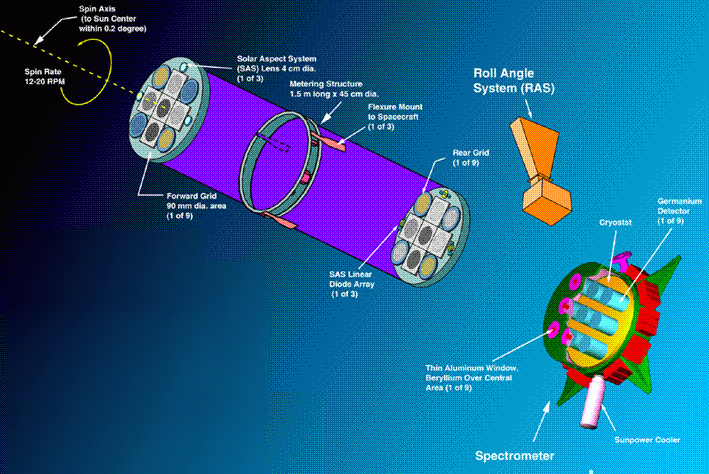
The HESSI scientific objectives will be achieved with high resolution imaging spectroscopy observations from soft X-rays to g-rays, utilizing a single instrument consisting of an Imaging System, a Spectrometer, and the Instrument Electronics.
The Imaging System is made up of nine Rotating Modulation Collimators (RMCs), each consisting of a pair of widely separated grids mounted on a rotating spacecraft. Pointing information is provided by the Solar Aspect System (SAS) and Roll Angle System (RAS)
The Spectrometer has nine segmented GeDs, one behind each RMC, to detect photons from 3 keV to 20 MeV. The GeDs are cooled to < ~75 K by a space-qualified long-life mechanical cryocooler to achieve the highest spectral resolution of any presently available g-ray detector. As the spacecraft rotates, the RMCs convert the spatial information from the source into temporal modulation of the photon counting rates of the GeDs.
The energy and arrival time of every photon, together with SAS and RAS data, are recorded in the spacecraft's on-board 2-Gbyte solid-state memory (sized to hold all the data from the largest flare) and automatically telemetered within 48 hours. With these data, the X-ray and g-ray images can be reconstructed on the ground The instrument's ~1° field of view is much wider than the ~0.5° solar diameter, so all flares are detected, and pointing can be automated.
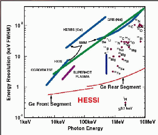
The enery resolution of HESSI (as a function of photon energy) is shown in Figure 3.2. For comparison, the resolution of instruments from on previous missions is also shown. HESSI has significantly better resolution than any previous mission.
HESSI is a Sun pointing spacecraft and is spin stabilized. Rotating at 15 rpm, the spacecraft spin axis is pointed within 12 arcsecs of Sun centre - the spin rate stability is < 4.5 arcseconds per second. The spacecraft inertia can be adjusted using the solar panels to align the imager with the spin axis. Other than this, magnetic torque rods are used for all pointing control. After launch, the spaceraft is able to acquire the Sun and spin up from any orientation without ground intervention.
HESSI observes the whole Sun and images are built up from Fourier components produced when the rotating collimator modulates a source. Images are reconstructed around a desired centre - to do this, it is essential to know accurately the pointing of the spacecraft rotation axis and the phase of rotation. This information is provided by the Solar Aspect Sensor (SAS) and Roll Angle Sensor (RAS) - see sections 3.2.4 and 3.2.5.
The imaging capability of HESSI is based on a Fourier-transform technique using a set of 9 Rotational Modulation Collimators (RMCs). Each RMC consist of two widely-spaced, fine-scale linear grids, which temporally modulate the photon signal from sources in the field of view as the spacecraft rotates about an axis parallel to the long axis of the RMC. The modulation (see Figure 3.3) is measured with a detector having no spatial resolution placed behind the RMC. The modulation pattern over half a rotation for a single RMC provides the amplitude and phase of many spatial Fourier components over a full range of angular orientations but for a small range of spatial source dimensions. Multiple RMCs, each with different slit widths, provide coverage over a full range of flare source sizes. An image is reconstructed from the set of measured Fourier components in exact mathematical analogy to multi-baseline radio interferometry.
HESSI provides spatial resolution of 2 arcseconds at X-ray energies below ~40 keV, 7 arcseconds to 400 keV, and 36 arcseconds for g-ray lines and continuum above 1 MeV (see Figure 3.4). The chosen spacecraft rotation rate of 15 rpm provides a complete image with the maximum number of Fourier components in 2 s, but spatial information from fewer Fourier components is still available on time scales down to 10's of ms, provided the count rates are sufficiently high.
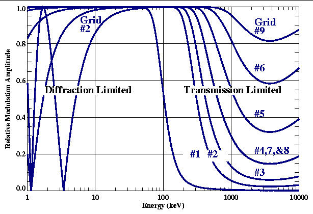
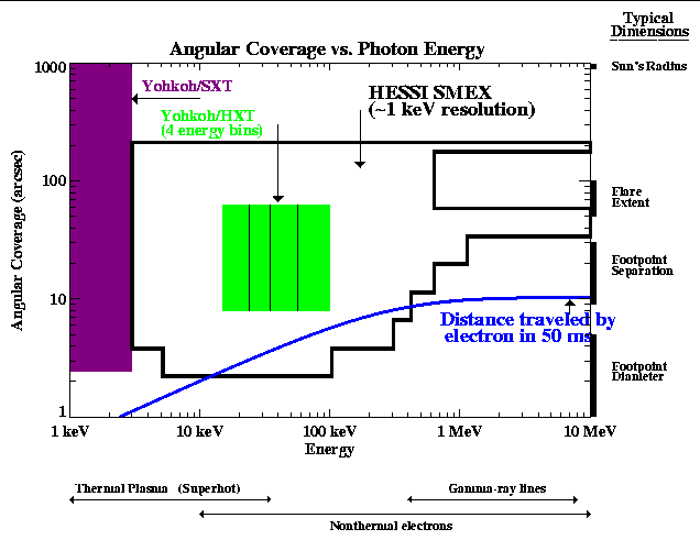
For HESSI, the separation between grids in each RMC is 1.55 m and the grid pitches range from 34 mm to 2.75 mm in steps of the square root of 3 (see the Table of grid parameters at URL http://hesperia.gsfc.nasa.gov/hessi/reference/Charts/Specs.html). This gives angular resolutions that are spaced logarithmically from 2.3 arcsec to > ~3 arcmin, allowing sources to be imaged over a wide range of angular scales (see Figure 3.4). Diffuse sources larger than 3 arcmin are not imaged but full spectroscopic information is still obtained. Multiple smaller sources are imaged regardless of their separation.
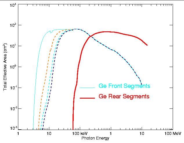
The grid material and thicknesses have been chosen to provide modulation to energies as high as possible consistent with maintaining a ~1° FOV. Only two maximum thickness grids were chosen, providing g-ray imaging while minimizing the loss in sensitivity for g-ray line spectroscopy. Thus, with the grid parameters selected, imaging is possible with 2.3 arcsec resolution to ~40 keV, 7 arcsec to ~400 keV and 36 arcsec to > 10 MeV (see Figure 3.4). Even allowing for the grid absorption, the effective photopeak area for high resolution g-ray spectroscopy is still ~80 cm2 at 1 MeV (Figure 3.7).
A metering structure is used to maintain the relative twist of even the finest grid pair to within one arcminute. This employs flexural elements to mount the grids to the grid trays and the telescope tube to the spacecraft in order to maintain the alignment following thermal and vibrational stresses. The approach was used successfully in the Hard X-ray Imaging Spectrometer (HXIS) on SMM, where the alignment requirements were significantly more stringent.
open solid angle (gt 30 keV)
TABLE of spatial and energy resolution??
The detectors used on HESSI are the largest currently available hyperpure (n-type) germanium detectors (HPGe) - 7.1 cm in diameter and 8.5 cm long. They cover the entire X-ray to g-ray energy range from 3 keV to 20 MeV with the highest spectral resolution of any presently available detector ( < 2 keV below 1 MeV to 5 keV at 20 MeV). The keV spectral resolution of germanium detectors is necessary to resolve all of the solar g-ray lines (with the exception of the neutron deuterium line, which has an expected FWHM of only 0.1 keV). It is also required to resolve the detailed features of the X-ray continuum spectrum such as the steep super-hot thermal component and the sharp breaks in the nonthermal component at higher energies.
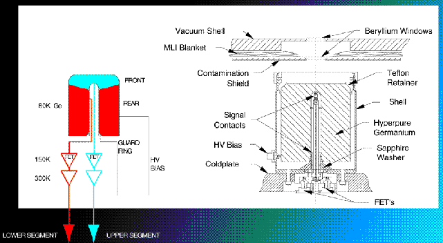
The Germanium detectors (GeDs - see figure 3.5) have three electrically-independent segments. The front 1 cm thick segment can measure hard X-rays up to 200 keV with low background. The rear 7 cm thick segment provides undistorted high-resolution g-ray line measurements, even in the presence of very intense hard X-ray fluxes in large flares (these are absorbed in the front segment). Finally, there is a < ~0.5 cm ``guard-ring'' at the bottom which increases the resistance of the detectors to contamination.
The Germanium detectors are cooled to their operating temperature of 75 K by a single electro-mechanical cryocooler. Studies at UCB have shown that radiation damage is significantly lowered by maintaining the GeDs at < ~75 K instead of the normal > ~85 K, and avoiding warmups above ~85 K and/or high voltage cycling. Additionally, a low-altitude equatorial orbit (38°) was chosen to minimize damage to the GeDs from the charged particles in the Earth's radiation belts. With these measures, the cumulative radiation dose to the Germanium detectors during a three-year mission lifetime is low enough to avoid noticeable radiation damage to the detectors. Thus, neither shielding nor detector annealing should be needed, although annealing (which can reverse the affects of radiation damage effects) is possible if necessary. The absence of a thick, and necessarily heavy, shield in this orbit, made the lightsat approach feasible.
Solar Flares have a wide dynamic range of intensity over the energy range below 100 keV, the energy range of interest for the HESSI front segments. Within that energy band there are both thermal and non-thermal phenomena of great scientific interest. The design goal for HESSI is to preserve as much of the non-thermal photons as possible for spectroscopy and image synthesis, while sampling the thermal phenomena with appropriate sampling techniques. Since the thermal phenomena range from the barely detectable to those that would saturate the detectors, special techniques must be employed. Typical thermal parameters may range from a temperature of 6 MK with an emission measure of 1048 cm-3 to 25 MK and 1050 cm-3, yielding a difference of over 8 orders of magnitude at 10 keV in the photon flux.
The original HESSI design in the SMEX proposal sacrificed much of the low energy sensitivity intrinsic to the germanium detectors in order to preserve full range spectroscopic measurements (possible only for photon flux rates below 50,000/sec) during all but the most intense flares. The design was modified during Phase A with the addition of a pair of moving attenuators over each detector to expand the dynamic range for imaging spectroscopy to include far fainter sources.
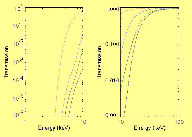
The system consists of two independent frames carrying one attenuator per detector. Each frame has two positions, open and closed. In the open positions, X-rays pass freely through openings in the frame which are slightly larger than the area of the front segment of each detector. In the closed position, each of the nine detectors is covered by an attenuating disk consisting of a thin layer of aluminum. The 9 disks on each frame are not identical, and are also different for the two frames. The two attenuators are designated as the ``Thin'' and ``Thick'' shutters, with the Thin shutter having less material than the thick shutter. There are four states of the full attenuator system: both Thin and Thick out, Thin in and Thick out, Thin out and Thick in, and both Thin and Thick in - these are designated with the shorthand notation 00, 10, 01, and 11. Details of the attenuator design and the material along the X-ray path with both shutters in the open position are given on the HESSI web pages at URL http://hesperia.gsfc.nasa.gov/~richard/shutter.html.
The attenuators have the greatest effect on low energy transmission, below 100 keV - see Figure 3.6, and the dashed lines for the front segments in Figure 3.7.
As a flare increases in intensity, the attenuation is automatically modified by switching the shutters in and out keeping the flux on the detectors below the maximum spectroscopy flux, while maximizing the sensitivity to the extent possible. The plate holding the attenuators is moved using Shape Memory Alloy (SMA) actuators. The switch only takes about a second, but since the SMA springs need to be cooled below their transition tempertaure (100 degC) before the opposite switch can be made, a waiting period of 5 minutes is imposed between opening and closing the attenuators. Note: the time of the switch is recorded in telemetry, but the photons recorded during this interval are currently not automatically rejected by the software and the user should be careful when accumulating across such changes.
The primary purpose of the Solar Aspect Sensor (SAS) is to provide high-resolution, high-bandwidth aspect information that is used for image reconstruction.
The SAS is similar to the aspect system on the HEIDI instrument, which demonstrated 0.5 arcsec performance at balloon altitudes. It consists of three identical lens-filter assemblies mounted at 120deg intervals on the forward grid tray. These form full-Sun images on three 2048 element × (13 mm)2 linear CCD arrays mounted on the rear grid tray. Simultaneous exposures of three chords of the focused solar images are made at selected periods ranging from 8 to ~60 ms. A digital threshold algorithm is used to select N pixels that span each solar limb for inclusion in the telemetry. Determination of these six limb crossings locations provide by the three subsystems define picth/roll offsets of the Sun in the rotating frame to better than 0.4 arsec.
When the spacecraft spin axis is pointing to within ~0.2° of Sun center, simple algorithms using the limb pixel numbers also provide real-time error signals with Ł 10 arcsec precision to the spacecraft Attitude Control System (ACS). Use of the SAS in this way for both imaging and pointing avoids problems of coalignment. The SAS is also used as a solar acquisition sensor with an effective radial field of view of 46 arcmin by the detection of a single limb in any one of the three diode arrays.
Although the aspect solution itself is independent of twist, the internal consistency of the three independent solutions (possible with the built-in redundancy) provides a continuous, highly sensitive measure of the relative twist of the upper and lower grid trays during flight. The SAS aspect requirement of 1.5 arcsec corresponds to a sensitivity to relative twist of 0.4 arcmin. During prelaunch coalignment tests, the twist determined by the SAS was calibrated against that provided by the Twist Monitoring System (TMS; modelled on a system developed for the SMM-HXIS instrument). This method would identify any twisting at the tray level - if twists occurred within a grid pair, this would be more difficult to determine.
For image reconstruction, a knowledge of relative roll is required at all times to 3 arcmin (3 sigma). Since all sources of torque on the spacecraft are weak, the required information can be obtained with a star scanner that samples the roll orientation at least once per rotation. Interpolation between measurements allows the roll orientation to be determined at intermediate times with the required accuracy.
The Roll Angle Sensor (RAS) consists of a 2048-element linear photodiode array and electronics (nearly identical to those of the SAS) behind an f/1.0, 50-mm lens. A sunshade limits the FOV so that a 30° band is swept out across the sky orthogonal to the spin axis. As the spacecraft rotates, each detected star generates a brief spike in the output of one or two pixels, the timing defines the roll orientation. For +2 magnitude stars, the detection signal-to-noise is 15:1. Allowing for Earth occultation and the recovery time from anticipated Earthshine saturation, at least one (and typically seven) such star(s) will be detected each rotation throughout the mission. Measurements of only one star, averaged over a minute, allow the roll angle to be determined to 2.7 arcmin (3 sigma).
Event Packets: HESSI data, whether a flare is active ot not, largely consists of event packets. These include the energy and arrival time of each event, together with information about the spacecraft aspect and rotation.
If the ondoard memory starts to fill up, a decimation algorithm throws out all but one of every N events in the front segments below a certain energy E, with N from 2-16. E and N are functions of both the remaining memory and the position of the attenuators. Decimation in the rear segments can be commanded as a routine way of keeping background (mostly photons from the Earth's atmosphere or cosmic diffuse background) from filling up the memory. For example, a high level of decimination can be commanded for times when HESSI is in the Earth's shadow.
The time tag of an event uses the last 10 bits of the time counter.
If the count rate is low enough that the last 10 bits
roll over between events, dummy ``time stamp'' events are inserted
so that the time on each events is not ambiguous.
Monitor Rates:
These are a separate kind of data packets - each packet consists of 10
1-second accumulations of a set counters for each of the 18 segments
(9 detectors, each with a front and rear segment). The counters include
countrates for the lower and upper level discimintators (LLD and ULD)
and the fraction of ``live'' results from the livetime strobe.
The information is used to check the health of the detectors and
to make livetime corrections to the data.
Note: Livetime affects only the intensity and not the
shape of the spectrum (see 3.3.2).
Fast Rates: Fast rates are produced when the count rates are very high. The data are count rates in four broad energy bands (all in the hard X-ray range). The pulses are sampled from the fast electronics chain. The rates for the three detectors (1,2,3) with the finest grids (and therefore fastest imaging modulations) are sampled at 16 kHz; the next three (4,5,6) at 4 kHz; and the three coarsest grids (7,8,9) at 1 kHz. Events are not shut off when fast rate data turn on. However, at these very high counts rates, the event data will naturally taper off due to very high deadtime.
The HESSI total effective areas for the front and rear detector segments are shown in Figure 3.7. The effects of the attenuators on the response of the front detector segments can be seen (dashed lines), these segments are sensitive to lower energy photons.
Figure of front and rear spectra from a typical HESSI detector ????
HESSI carries small onboard radioactive sources (137Cs) which produces a line at 662 keV, far from any line expected to occur in flares or in HESSI's variable background. The known intensity of the line makes it possible to monitor changes in the efficency of the detectors, such as might be caused by radiation damage. The count rate from the source is so small that it can only be detected in spectra accumulated over many hours and therefore does not affect the observations.
Because the detectors are cooled, the effects of radiation damage are expected to be minimized.
Pile-up Rejection: Closely spaced events can cause pulse pile-up in the analogue electronics. This is because the electronics have not finished processing one event before the next one arrives. To reduce this problem, events less than 6 ms apart are rejected outright, while for those with seperations between 6 and 9 ms, the second event is rejected - this is affected by the tail of the first event.
Pile-up results mainly from lower energy photons. In the front segments, events below about 6 keV (which don't trigger the lower level discriminators in the fast electronics) can pile up unrestictedly on other events. Pile-up adds a wedge of counts at the lower end of the spectrum and can also add peaks to the spectrum at higher energies that are ``ghosts'' of lower energy peaks.
Pile-up correction is an iterative process based on the shape of the
raw spectrum and knowledge of the countrate and measured livetime.
It corrects the shape of the spectrum, and removes the extra higher
energy peaks.
For the majority of flares, pile-up correction will be unnecessary, and
for most of the remainder, first-order corrections will suffice.
Livetime: Livetime is independent of energy, and the livetime correction changes only the overall magnitude of the spectrum (i.e. photometry) rather than the spectral shape. However, livetime corrections must be applied consistently to all detector segments to avoid indirectly modifying the shape of the spectrum.
The livetime of a detector is simply the probability that one additional count, put in at a random time, would in fact be recorded. The livetime signal for each segment is derived from flags from different parts of the electronics indicating they are busy. The signal is sampled at 1 MHz and the livetime reported in the monitor rates is the fraction of the sample strobes that are clear. Note: Deadtime is (1.-livetime), the percentage time that a circuit is ``tied up'' by other events.
Because the pile-up circuit can sometimes veto both events, there is a loss of livetime that cannot be measured just by sampling the pile-up rejection logic line. The livetime correction routines therefore do not use the ``raw'' livetime measurements as reported, but a corrected livetime, which is somewhat lower.
The maximum event throughput is 25-30 thousand count per segment per
second and is reached at about 50% livetime.
Background Subtraction: HESSI is an unshielded, high-background instrument and it is therefore necessary to subract background even in the case of bright flares.
The simplest way to estimate the background is to average spectra from just before and just after a flare. This is the default method provided in the software, and the user is asked (see Section ??) to pick intervals that should be used as background from a lightcurve (countrate vs. time).
In cases when the flare lasts the better part of an orbit, or occurs just
after sunrise, or just before sunset, this technique is difficult to apply.
Using background from the orbits before and after the flare,
at the same orbital phase as the flare, is one way to solve this problem.
Other techniques are being developed.
Image events: When a gamma-ray event moves through the detector, the hole and electron clouds liberated in one segment can induce charge in the other segment. The event is correctly detected in the first segment, but an image event can also be detected in the other (empty) segment. The difference is that the image charges reverse sign in the empty segment as the clouds approach the electrodes of the segments in which they are actually moving. The result is that the image signals in the empty segements are bipolar in shape and integrate to zero.
The HESSI electronics only sample for a finite time (a few micro seconds), and a small amount at the very end of each pulse is not counted. The sampled pulse is normally negative (???), and since it is the negative part of the bipolar pulse that comes last in the empty segment, the result is a very small, positive residual from the bipolar signal. In other words, a 1 MeV event detected in one segment will create a simultaneous (but false) event of a few keV in the other segment.
Thus, you may also hear image events referred to as ``bipolar pulses'' or
``false coincidences''.
Other concidences: There are two other ways events can be coincident between two segments (or two detectors): there could be real energy deposits in both segments from the same initial photon or cosmic ray (``true concidences''), or there can be separate photons that arrive at nearly the same time by chance (``accidental coincidences'').
The simplest way to do spectroscopy is to throw away all coincident events - defined as events within N binary microseconds of each other (where the best value of N is 4 or 5). However, in order to detect faint gamma-ray line, you may want to include front/rear coincidences, and concidences between adjacent segments (the software has a flag for this??). Also, when the countrates are very high, you may not want to reject coincidences at all since a large fraction of the events will be accidental coincidences.
At moderate countrates, true coincidences can be separted from image events by precise relative timing of the two events.
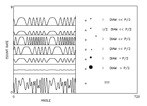
As the HESSI spacecraft rotates, the signal produced by a source is modulated by the rotating grids - the way it is modulated changes depending on the source position, intensity and size. In Figure 3.8, the right hand panel shows single sources of different sizes and intensities at different locations relative to the spin axis (marked with a ``+''), and the left hand panel shows the resulting modulation patterns.
The top line shows the modulation resulting from a source whose diameter is much less than half the separation distance (P) from the axis of rotation. If the intensity of the source is halved (2nd line), the amplitude of the modulation is reduced. If the the distance of the source (of original intensity) from the axis of rotation is changed (3rd line), the frequency of the modulation pattern is modified. When the source is kept at the same distance as the top line, but rotated around the axis of rotation (4th line), the phase of the pattern shifts (although its form is the same at the first line). When a source is placed at the same location as the top line, but its size increased (lines 5 and 6), the amplitude of modulation decreases about its mean value until (when the source size exceeds half the seperation distance) is it barely visible.
Of course, the reality of actual observations mean that sources have complex shapes of non-uniform intensity and the resulant modulation pattern is much more complex (e.g. the bottom line). The image reconstruction techniques try to recreate the original source structure using the information contained in the modulation patterns observed in the different collimators.
Also see the explanation about image reconstruction on the Web pages under URL http://hesperia.gsfc.nasa.gov/hessi/hessi_show_image.htm.
It is important to keep in mind some of the limitations of the imaging technique when recontructing HESSI images and analyzing the data.
At first, it might seem that the best results are obtained using all the subcollimators since this results in the largest number of total counts available for constructing the image; however, this is generally not the case:
| Collimator | 1 | 2 | 3 | 4 | 5 | 6 | 7 | 8 | 9 |
| FWHM | 2."3 | 3."9 | 6."9 | 11."9 | 20."7 | 35."9 | 62."1 | 107" | 186" |
These considerations suggest that weighting among selected subcollimators could be very useful, and can certainly help backprojection and CLEAN image quality. Two possible weighting schemes are available.
Aside from the choice of subcollimators which will optimize a given image, there are spectral considerations for the imaging to be aware of as well. In some ways, it is difficult to separate the spectral aspects of the imaging from the imaging itself. This leads to a few facts the user should be aware of. The first consideration then is imaging spectroscopy. Many users will want to make images of fields which contain more than one source and then wish to obtain a spectrum of each source. The current way to approach this task is to make images in a number of different energy ranges and then add up the counts in each source to construct the spectrum of the sources.
A related consideration then is just how broad an energy range to use when constructing an image. Since you get more counts and hence higher signal-to-noise ratio, it might be assumed that the broader the energy range, the better - however, this is not necessarily the best choice. The HESSI imaging software uses all the photons detected between the specified energy range to determine the modulated light curve from each detector for the specified time interval. The software then assumes a mean energy for this energy range for computing the expected response of the instrument which is applied to the data to compute the image. However, since the modulation patterns themselves are a function of energy, there is no unique instrument response that works for all energies. Therefore, it is not a good idea to construct images with an arbitrarily wide energy range.
One way to attack this problem is to make several images with smaller energy ranges and compare them. As long as the structure of these various images remains the same, it is probably OK to then make a final image encompassing the whole energy range.
An important aspect of image analysis using HESSI data is to be able to decide which features in the image can be trusted. Some factors to consider when trying to judge which features of an image to trust are the following:
A. A reasonable fraction of the total counts should be in the feature of interest (a smaller fraction is more susceptible to systematic calibration errors). Counting statistics - statistical signal to noise in the peak of a backprojection map is proportional to SQRT(totalcounts);
B. Image morphology - too complex an image structure may not be real (simpler is better);
C. Unusual source variability: if the source is changing rapidly in relative intensity across the image, this could produce confusing results;
D. Instrumental effects could also affect the image quality. In addition to any hardware or software anomalies, these might include:
Any unusual characteristics of the aspect solution should also be considered.