|

| - First steps - In detail - Software notes - Examples
|
GIS users guide - in detailAssociated software note is #55, the User Manual. This page contains information for the experienced GIS user. Please click on a topic in the list below. If you cannot find the information you require please contact Lucie Green or visit the Examples link on the left hand side.
- GIS data
GIS data Unlike the NIS, GIS is astigmatic and the whole of the spectrometer slit is used to produce the spectra. Data in all 4 detectors are gathered simultanously. To collect data from an area larger then the GIS slit size, the scan mirror or the slit can be moved.
Reading GIS data into SSW IDL GIS data is read into the IDL session in the form of a Quick Look Data Structure (see below).
The Quick Look Data Structure (qlds) The quick look data structure is the standard format of data used by the CDS software. It contains the spectral data, some wavelength calibration information, ancillary information about spacecraft pointing, and much more in a hierarchal structure. To browse information in the qlds type: IDL> help, qlds, /str or IDL> help, qlds.header, /str or IDL> print, qlds.hdrtext Please note that the qlds is CDS specific and CDS routines must be used with them. For example, to copy a qlds the normal IDL command cannot be used, instead type: IDL> qlds = copy_qlds(a) Quick look at the data The routine dsp_menu allows a quick look at the raw or processed GIS data. IDL> dsp_menu,qlds A menu is brought up and under 'Data display modes' the user can select, for example, to produce a 'Snapshot' of the data or a 'Full detector view'. Under the latter option there is a choide to 'Mark lines' and over plot pre-set line lists. It is also possible to identify lines and measure their positions and intensities. To display a snapshot of the data in all four detectors without going via dsp_menu type; IDL> cds_snapshot, qlds [, /spectra, /log] This plot will display the spectra for a sit and stare study, or an image if several rasters have been taken. For rasters set the /spectra switch to force a spectra (and not an image) to be displayed.
Extracting data from the Quick Look Data Structure To extract data from the (calibrated) qlds the routines gt_windata and gt_spectrum can be used. IDL> data = gt_windata(qlds, window [, /nocheck, /quick, /nocopy, /nopadding, errmg=errmsg]) Window is just the GIS detector number minus 1. So, for example, to extract data for GIS detector 3 type: IDL> GIS3data = gt_windata(qlds, 2) The data are returned are a floating point array of up to 4 dimensions:
To obtain a description about the data in GIS detector 3 the gt_windesc routine can be used IDL> GIS3desc = gt_windesc(qlds, 2) The returned structure GIS3desc gives the units for the data in GIS3desc.units, the flag for missing data in GIS3desc.missing and the wavelength range in GIS3desc.wavemin and GIS3desc.wavemax. Displaying and finding ghost details The routine ghost_plot_one displays data from one GIS detector and shows the regions of the spectrum which contain ghosts. It can be used to check whether a line is ghosted (ie. a true spectral line which has additional ghosted counts) or is a ghost line (ie. a false spectral line). Note: the ghost_buster routine can be used to move to original location, or remove, ghosts in the GIS data. IDL> ghost_plot_one, qlds, detector_no [,/sample, /nm, /angstroms,/logscale, /pixels, waverange=[min, max], /cross_cor] The above routine allows switches to modify how the data are plotted. For instance, waverange can be used to zoom into a particular region of interest, by specifying a minimum and maximum wavelength to be plotted; and /sample plots a sample theoretical spectrum for comparison of where the spectral lines should lie. The routine also plots the observed spectrum shifted by one spiral arm to longer and shorter wavelengths (called red and blue shifted) to help identify ghost locations. To check whether a line is ghosted or is a ghost, first look to see if it is in the shaded region of the output from ghost_plot_one. If it is, check to see if there is a corresponding line in the theoretical spectrum. If there a corresponding line it is likely to be OK, but check also in the blue or red shifted spectra to see if the observed line could have additional ghosted counts. If there is no corresponding line in the theoretical spectrum check to see if there is corresponding line in the blue or red shifted spectra. If there is, it strongly suggests that the line may be a ghost and that the counts need to be returned to their original position. Ghost information files and structures Every GSET has an associated ghost information file which contains the pixel locations of regions which are affected by ghosts, but which are not automatically corrected by ghost_buster. The ghost information files are located in the same directory as the other GIS calibration data; $CDS_GIS_CAL_INT. Also in this directory are the ghost information structures which are used by ghost_buster to restore ghosts automatically.
Ghost correction In total there are 3 ways to make corrections for ghosts in the data using the routine ghost_buster:
Pointer: to check whether the region of interest in the spectrum has ghosts, the ghost_plot_one routine can be used. See 'Displaying and finding ghost details' for more information.
Plotting GIS spectra The routine gis_plot plots a summary of the GIS data from a detector of choice. It will plot raw or calibrated data from the qlds. IDL> gis_plot, qlds, detector_no [, /logscale, waverange=[min,max] ] The plots can be made in Angstroms or nm.
Line fitting The routine gis_fit can be used to automatically fit clearly identified lines in the GIS spectra. This routine can be used on calibrated or uncalibrated data. In the latter case, the routine will smooth the data and make ghost corections for the unblended ghosts. IDL> gisfit = gis_fit(qlds, /plot) If the /plot switch is used the progress of the fitting can be followed. The output 'gisfit' is a structure which contains the line intensities, amplitudes and widths along with the associated uncertainties. To obtain information on the structure type IDL> help, gisfit, /str the following is returned:
HEADER STRUCT -> Anonymous Array[1]
These structures hold the information for each line and can then be further interigated.
CHIANTI consists of a databse of atomic data and IDL procedures for for calculating spectroscopic emission line intensities at wavelengths greater than 50 Angstroms from optically thin astrophysical spectra. It is freely available and contains the most up-to-date atomic data including energy levels, transition probabilities and electron collisional excitation rates.
In order to use CHIANTI within the IDL session the correct branch of the software tree must be loaded either when initialising IDL
IDL> setssw cds chianti
or from within IDL
IDL> ssw_path, /chianti
For more information on CHIANTI and for a User Guide see the CHIANTI homepage.
The main IDL routine for deriving differential emission measure (DEM) analysis of EUV spectra is chianti_dem which uses the CHIANTI database.
Electron density
Density-sensitive line ratios are used to obtain the electron density in the corona. One ratio suggested for use are the two Fe XIII lines at 202 A and 204 A.
Step 1: Density-Ratio Calibration
There are many ways to do the density-ratio (intensity ratio of two lines) calibration, two ways are suggested here. One is "by hand", using the CHIANTI routine ch_ss which generates synthetic spectra. The second way is automatic using the routine chianti_ne, which is designed to calculate and plot density sensitive line ratios, and is faster and easier to use. The calibration is a bit time-consuming but only needs to be done once.
The first method: Run the routine ch_ss
IDL> ch_ss
You will see the CHIANTI Spectral Synthesis Package window. Set the Wavelength, Const. Density, Ioniz. Fraction, Ion(s), Line(s) and Temperature to the values required and click Calculate intensities at the right.
For example, if the Fe XIII 202 A and 204 A lines are used, the following may be set may set:
Wavelength min.: 200, max.: 205;
Click the Calculate intensities.
When the calculation is finished, go on to select the proper Abundances, in this case, for example the sun_coronal.abund. Click the Calculate and plot.The spectrum of Fe XIII from 200 A to 250 A can then be seen
Click the peaks that are required, for example, the 202 A and 204 A lines, and record the intensities shown in the window at the bottom. Change the Const. Density as required, and record the densities and intensities. This is the calibration data.
An alternative method: Run the routine chianti_ne
IDL> chianti_ne
In the window, select the min. and max. wavelengths, the ion, the temperature, and density region you would like to plot. Then Calculate line intensities, and Plot ratio. Use the Save button to save the ratio data to file (e.g. 'fe13ratio.CH_NE'). This file may be restored in later IDL sessions:
IDL> restore, file='fe13ratio.CH_NE'
Then, we finally get the arrays of density and ratios: NE_RATIO.DENSITY, NE_RATIO.RATIO. Save them into a text file.
The results of the two methods above are the same; a list of the ratio and density. To be read smoothly by the program which calculates the densities they should be recorded in the following format. It begins with N, the number of calibration data, followed by N lines of the density and ratio.
N
The calibration data for the two Fe XIII lines mentioed above cane be downlaoded here (fe13.cal).
Step 2: Make the Ratio Map
This method can be used on GIS data from studies which raster over small areas.
Read in the fits file as a qlds, and calibrate the data (gis_smooth etc.) Use the functions gt_windata (), pix2wave () to get the spectrum and the wavelength calibration.
IDL> g1=gt_windata (qlds, 0)
IDL> xcfit_block, w1, g1, 1./(g1>0.01), fit, -100., result, residual
The input, fit is an array which tells the routine which part of the spectrum to work on. The '-100' just tells it the missing line as mentioned. The 'result' and 'residual' are the two output arrays.
In the xcfit_block windows, click the Adjust button first to adjust the max. and min. values etc. and then click the Calculate (choose that from global initial values) to go on. It is possible to download an existing saved 'fit' array here (fit_fe13.sav). Then you only need you restore it before you load the xcfit_block. It is suggested that you have a look at the width of the gauss peak before going on to Calculate.
Then exit xcfit_block, and save the results to file 'fe13.txt':
IDL> openw, 1, 'fe13.txt'
IDL>plot_image, reform(((RESULT(3,*,*)-RESULT(6,*,*))*RESULT(5,*,*))/((RESULT(0,*,*)-RESULT(6,*,*))*RESULT(2,*,*)))
A procedure is available here (gt_ratio.pro) which contains all the steps necessary to detemine the density. A saved fit array is also needed and can be found here (fit_fe13.sav). If you also like to have an example, you may also download this (fe13.txt).
The GIS records spectra over small regions of the Sun. In order to check the pointing of an observation use the gt_point routine. There is also an offset in the pointing which must be corrected for (see below).
IDL> print, gt_point(qlds)
The pointing is returned in arcseconds from the solar centre in X and Y.
Other routines that could be used include dsp_point and dsp_raster.
Pre-July 1998, there was a small offset in the GIS pointing; after that date the GIS pointing, relative to NIS,
has been 20.2" to the south for the default roll angle.
This offset varies with SOHO roll ange. With normal roll angle (ie. no roll angle)
the offset is maximal since the offset is in the N-S direction. For 180 deg. roll the offset changes sign.
The header of the data does not correct the coordinates for the offset.
and that applies also for positions given in the data header or the Quick Look Data Structure.
Due to the problem with the main antenna SOHO has been changing it's default roll angle of 0 degrees twice a year to 180 degrees, i.e., north becomes south and east becomes west.
To find information on SOHO's roll angle
IDL> print, get_soho_roll ('11-mar-2005')
The returned value is the roll in degrees in the clockwise direction starting from north.
Even when the offset in the pointing has been corrected for, between consecutive NIS and GIS data, or between
two programs that involve GIS repointings, there remains a random pointing uncertainty of about 5 arc seconds.
A pointing study (Kuin and Del Zanna, 2006) shows data from which one can see, that for most cases the random
pointing changes are within 3 arc seconds, though.
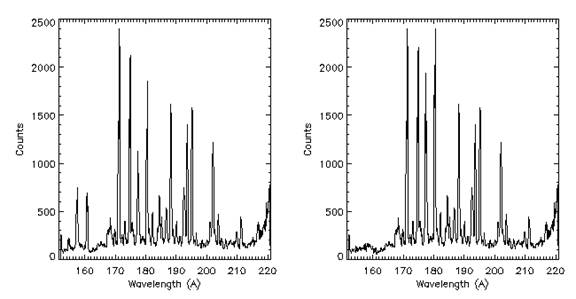
The nature of Micro-channel Plate (MCPs) detectors results in a reduced efficiency in the production of secondary electrons over time. This means that there is a gradual loss in gain (number of incident photons versus charge output). The degradation depends on total charge extracted from the MCP, not the rate, and is seen in the regions of the brightest spectral lines.
This effect is known as long-term gain depression (LTGD).
A 'flat field' for GIS detector 1 produced using a filament above the detector which produces a cloud of electrons to mimic photons incident on the MCP. The dips due to decreased sensitivity at the brightest spectral lines are clearly seen.
The LTGD produces 2 effects on the shape of the spectral lines; a broadening and a 'dip' in the peak line intensity. These effects have been studied over the duration of the mission. Click here to see the changes to the Fe IX 171 Angstrom line.
This effect is countered by occasionally raising the voltage across each MCP stack and by applying corrections to the data. The routine gis_calib makes the LTGD corrections.
One line summaries of all CDS software routines (GIS and NIS) can be found here. For more information on the routines type:
IDL> doc_library, 'routine_name'
|