First steps in processing GIS data - all you need to know

GIS data are stored and distributed in FITS format. In order to prep and analysis the data within IDL something called a quick look data structure (qlds) is produced when the GIS data is read into IDL. Something about the GSETs as they are mentioned in the text below.

Once the qlds is processed the spectral can be extracted.

Firstly load in your GIS data. If it is contained in an archive at your instition you can use type 'xcat, QL' to access the catalogue and produce a qlds. If you are using files stored in your own directory they can be loaded in by:

IDL> qlds = readcdsfits('s4384r00')

There are very few steps required in processing GIS data. They include corrections for:

• Fixed patterning - a displacement of some counts in the emission lines producing 'spikey' line profiles. Total counts in a line not affected.
• Ghosting - Displaced spectral lines caused by an effect in the GIS detectors.
• Intenstity calibration - Caused by non-linearities in the detectors and their electronics.
• Wavelength calibration - Translates GIS positional counts into wavelengths.
• Correction for the pointing offset - Since July 1998 GIS pointing is offset 20.2" south of NIS.

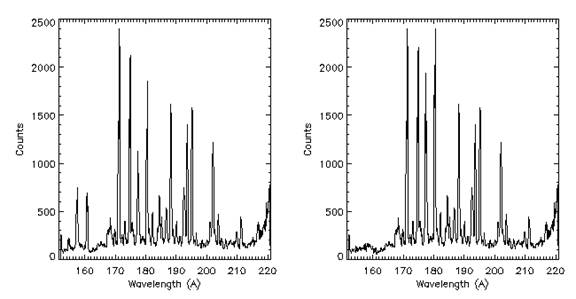
1. Fixed patterning

Fixed patterning is an effect caused by the interaction of the GIS digital electronics and the analgue detector read-outs which makes the spectra look 'spikey'. It is removed with the procedure gis_smooth. In some parts of the spectra it is very pronounced.

A boxcar smooth of the data will reduce the effect but increases the line widths. So, a convolution with a Hanning function is used in the gis_smooth. This function preserves the total counts in the spectral lines without introducing artefacts in the background or increasing the line widths.

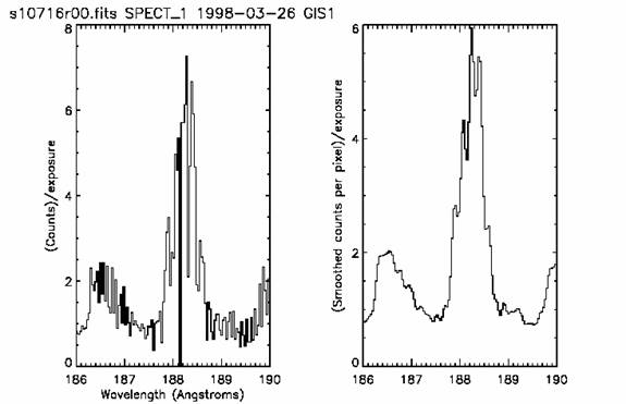A plot of the data around the Fe XI line showing the fixed patterning (left plot) and the smoothed data (right plot).

To smooth the data once you have read it in as a qlds

IDL> gis_smooth, qlds [,smoothsize=size]

The option smoothsize exists to change the size of the function used. The default is smoothsize=7 which works under normal circumstances.

Note: missing data are estimated automatically within the procedure and then marked as missing again after the smooth has been applied. It is therefore not recommended to replace missing data separately before using any GIS processing software.

2. Ghosting

Electronic noise in the GIS detectors causes counts to be shifted between spiral arms. This can produce two things:

• False spectral lines
• Increase in intensity of existing spectral lines

The counts shifted by this effect are known as ghosts and it is possble to deduce which regions of the spectrum are affected.

The programme used to display and/or remove ghosts is called ghost_buster.

For the new user the programme can be used in 2 ways (the second way is recommended):

• To REMOVE ghosts and return regions of the spectrum which are not affected by ghosts (ie. it removes ghosted areas so the qlds is returned with missing data).

  IDL> ghost_buster, qlds, /free

• To identify and automatically MOVE ghosts which are not blended with other lines, one detector at a time so that the full spectrum is retained.

  IDL ghost_buster, qlds [, hardcopy, /nm, /plot]

For the advanced user a manual ghost correction can be made. See the 'In detail' section of the GIS User Guide.

3. Intensity calibration

The intensity calibration corrects for the non-linearities in the detectors and their electronics.These corrections are small and made with a programme called gis_calib.

IDL> gis_calib, qlds [,errmsg=errmsg, /setmissing, /quiet, /steradian_m2, /arcsec2_cm2, /HeII/]

The data is returned as corrected counts per second per pixel by default. To convert to photons per second per solid angle per area use the /arcsec2_cm2 or /steradian_m2 switches.

The routine checks to make sure that ghost_buster has been run for all the detectors. If ghost_bsuter hasn't been run the /setmissing switch can be used to mark the ghosted data as missing. This switch can also be used to mark smaller areas of the data missing if they cannot be calibrated for other reasons (eg. a strong line which is too bright for the gain depression calibration or count rates too high for the electronic dead time corrections).

The region around the He II 304 A line is so bright that by default it is marked as missing. This is because in this region the detector efficiency is less than 1% of the original efficiency due to the brightness. To override this use the /HeII switch.

4. Wavelength calibration

The wavelength to pixel relation for GIS spectra depend on many factors including the slit used and the look-up table applied to convert the spiral pattern to a one-dimensional spectrum. Therefore each spectrum with a different GSET requires a different wavelength calibation.

The wavelength calibrations are automatically applied to the GIS data when the FITS data are read in as a qlds. The calibration information can be accessed by the routines pix2wave and wave2pix. To obtain a wavelength array applicable to a particular data window use the routine pix2wave.

IDL> wavelength = pix2wave ('GIS1' , findgen(2048))

Note: The wavelength calibration varies with each GSET used. So in order to compare two GIS observations that used different GSETs it is necessary to reload the wavelength calibration. See the 'Examples' section for information.

One line summaries of all CDS software routines (GIS and NIS) can be found here. For more information on the the routines type:

IDL> doc_library, 'routine_name'

5. Pointing Correction The pointing of the CDS has an uncertainty of several arcseconds from one program to the next. In addition to that random pointing uncertainty, there exists since the loss of SOHO attitude in July 1998 a mean pointing offset from GIS with respect to NIS of 20.2 arcseconds to the south.

The pointing offset has been determined by processing all available limb data for GIS and comparing to NIS data taken mostly at the same day. A report has been prepared of the study Pointing study PDF file.

At present, the user is expected to make the necessary corrections to his/her data him/herself. In the future a solarsoft routine will be made available to make that easier to do.