Unlike the NIS, observations with the GIS are astigmatic, and the whole of the spectrometer slit is used to produce the spectra. To cover an area larger than the normal GIS slits (2"x2", 4"x4", and for observations away from the solar disc 8"x50") the scan mirror and slit are moved over an area of up to 4 arc minutes. Data from all four detectors are gathered simultaneously, and although the minimum integration time is 1 second per pointing, it takes about 15 seconds to transmit the data. Thus to cover an area of 20"x20", using the 4"x4" slit and 50 second integration time per position takes just over 20 minutes. Because the GIS electronic encoding is sensitive to the incoming count rate, different GIS set-up (GSET) parameters are needed for different expected count rates. Much of this selection process is automated when the observation is uplinked to the spacecraft, although the observer must specify the solar `zone' beforehand. The zone is a rough description of the solar activity expected in the observation. It can be one of:
off limb: not on the solar disk. The expected maximum detector count rates for these areas are below 5 counts/second/pixel. quiet sun: any quiet area of the sun, including coronal holes. The expected maximum count rates are 20 counts/second/pixel. active region: active regions, including those on the limb. The expected maximum count rates are above 20 counts/second/pixel.
Once the zone and other observation parameters (raster size, slit, exposure time, exact location, etc.) are determined, the CDS planner at the Experiment Operations Facility can insert the GIS observation into the current plan. The combination of zone and slit selected will prompt the CDS planner to choose an appropriate GSET. The GSETs themselves are pre-determined from special (raw) observations made with the GIS. A number of raw observations for each zone, each slit, each detector and for various high voltage settings, are examined by the GIS team at MSSL and the best selected to produce the current set of GSETs. The raw files associated with each GSET are also used to produce ghost information structures and files. These enable likely ghosting regions to be identified, and in many cases corrected for automatically.
The CDS mission dataset can be browsed interactively using the powerful widget based `xcat' routine.
A lot of progress can be made using this routine, such as displaying images and spectra. It is a good idea to play with the menus at this stage if you haven't already done so. For example try selecting `GIS only' from the `Detector' menu, and put the required dates in the `Start Time' and `Stop Time' fields, and try selecting each of the read file options.
It is also possible to investigate the databases directly using the `list_exper' routine. This route is particularly useful when you want to find data automatically within one of your own IDL programs.
The output `obs' is an IDL structure which contains full details of the observations which CDS performed between the selected times. You can get an idea of the contents by typing:
You can use simple logic to select particular observations. For example to select all the GIS observations performed in the selected time interval:
The qlds contains the spectral data, some wavelength calibration information, ancillary information about spacecraft pointing, and much more in a hierarchal structure similar to that obtained using the LIST_EXPER routine (mentioned in the previous section). It is possible to browse all the information in the qlds with the following
This will display the following:
QL_ID DOUBLE 1.0570199e+009 QL_NO INT 1 HDRTEXT STRING Array[481] HEADER STRUCT -> HDRX Array[1] DETDESC STRUCT -> GISXX3 Array[4] BACKGROUND INT 0 WAVECAL STRUCT -> GIS_WAVECAL Array[1] DEL_TIMEDATA DOUBLE Array[20] DEL_TIMEDESC STRUCT -> AUX2 Array[1] INS_XDATA FLOAT Array[20] INS_XDESC STRUCT -> AUX2 Array[1] INS_YDATA FLOAT Array[20] INS_YDESC STRUCT -> AUX2 Array[1] ...
The structure can be investigated further in the following fashion.
This will display the GSET for this observation. This embedding of information with the data is a powerful method of distributing the data and greatly simplifies the analysis process, making easy to quickly display and analyse the raw data. For example to plot all four GIS data windows you can use the routine `cds_snapshot':
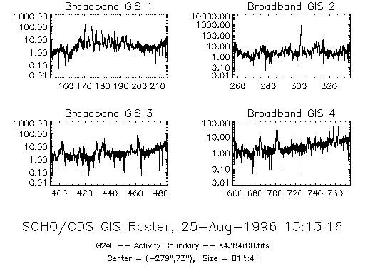
Figure 1: cds_snapshot of GIS data, using the /log switch. The salt and pepper noise which can be seen over this data is due to fixed patterning (described in section 4.1). This plot displays spectra since the G2AL study is a sit and stare study. For rasters, cds_snapshot will display an image, unless the /spectra switch is used.
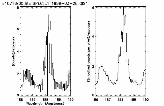
Figure 2: A plot of the data around an Fe XI line from study 10716, showing fixed patterning (left plot), where data shows large variations from pixel to pixel. The right plot shows the same data after running gis_smooth.
To smooth the data within a qlds use:
The option smoothsize exists to change the size of the function used, but the default (smoothsize=7) works under normal circumstances. To assist with the smoothing operation, any missing data in the data set are estimated automatically, the smooth function is applied, and then the original missing data marked as missing again. It is not recommended to replace missing GIS data separately before using any of the GIS processing software; it is taken into account already by the programs.
An effect in the GIS detectors is the presence of `ghosts'. These are displaced spectral lines, or parts thereof, caused by an ambiguity in the encoding used by the electronics.
The routine ghost_buster is used to remove or return ghosts in the GIS data. When the GIS is in raw data mode, it transmits the data from one detector as a series of coordinate pairs from the detectors. When these coordinates are plotted they form a spiral (see the GIS Instrument Guide) where the spectral dimension lies along the length of the spiral, and the intensity is the number of counts at each position along the spiral. To translate these pairs into spectral position, a Look up Table (LUT) is used as part of the on- board GIS processing. The parameters that define the LUT, plus the high voltage setting, form the GSET mentioned earlier. Every GSET includes a different set of LUT parameters, and the LUTs are calculated by the on-board GIS processor for each detector immediately before the first observation using that GSET. The ambiguity (or ghosting) in spectral data does not occur over the whole spectral range, but where the thin spiral arms broaden and overlap each other. If a spectral line is ghosted, it is confined to occur only at specific locations in adjacent spiral arms.
These characteristics are used in ghost_buster to restore the ghosts to their original locations. The counts in a ghost must be added to the counts at the original location to produce the correct line intensity. In ghosted areas, which cover 40% to 50% of the data, it is easier to separate the original line from ghosts where there are no blends. Thus ghosted areas in quiet sun observations are easier to correct than in an active region; although the unghosted areas remain unaffected for all observation zones.
This routine allows switches to modify how the data are plotted. For instance, waverange can be used to zoom into a particular region of interest, by specifying a minimum and maximum wavelength to be plotted; and sample plots a sample theoretical spectrum.
The routine first adds all the data from an observation into one spectrum per detector, then plots the data with information to help find possible ghosts. Figure 3 was produced using:
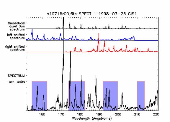
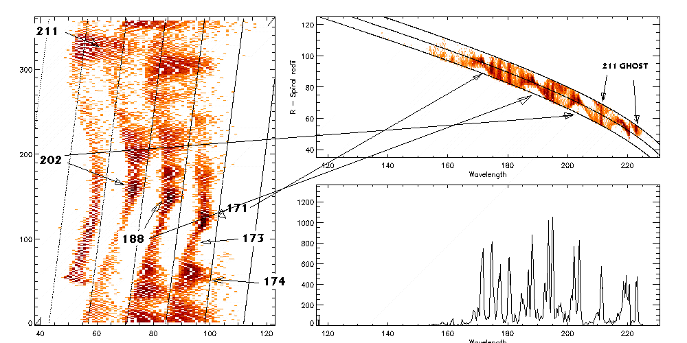
Figure 3: output from ghost_plot_one, (top-top) theoretical quiet sun spectrum, (top-middle) left shifted spectrum, (top-bottom) right shifted spectrum. (Bottom) Spectrum to be de-ghosted, with likely ghosting regions shaded. The areas of the resulting plot are described from the top:
The output from ghost_plot_one (Figure 3) can be used to check whether a line is ghosted, or itself is a ghost. Suppose we have seen a line, and want to check it; for example there is a spectral line on the plot between 160 and 161 (these ghosts are now corrected automatically by default, since they are located in non blending regions - see section 4.3). This line is in the ghosting region defined by the shaded region on the plot. The first check is to look at the `theoretical quiet sun spectrum'; it shows that there are no lines at this location. This may be a fault with the theory; however further checking shows that the `left shifted spectrum' also has a line at this point. This strongly suggests that the line at about 160 is a ghost and needs to be pushed to the right to correct the line. The manual ghost correction software explains the process of moving the line in more detail, as well as overlaying a `ghost cursor' on the plot. This cursor shows exactly where lines would come from if they are ghosts. Alternatively, if we are familiar with this area on the solar spectrum we know there is a FeXIII line at 202 (see Appendix C). To see whether this line needs correcting, first notice that it is a clear area of the plot, i.e., not in a ghosting area. Neither the left nor right shifted spectra show lines at this point, and thus this line is free from ghosts.
The ghost information files contain the pixel locations of ghosting regions which aren't corrected for automatically by ghost_buster. All GSETS have a ghost information file, which is stored with the other GIS calibration files located in the $CDS_GIS_CAL_INT directory. Also located in this directory are the ghost information structures, which are used by ghost_buster to automatically restore ghosts. 4.3 Ghost Correction There are now three modes for ghost correction: automatic, manual and ghost free. By default ghost_buster works in automatic mode. This automatically corrects for most ghosts where they are not coincident on other lines and are resolvable.
This corrects for about half of the ghosts (or 70% of the data, see Figure 4).
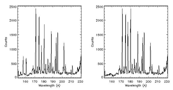
Figure 4: Ghost_buster automatic restoration of ghosts. (Left) uncorrected averaged smoothed spectrum. (right) The same spectrum corrected using ghost_buster in automatic mode. This works well for quiet sun observations, restoring almost all lines.
To correct the remaining ghosts, where the ghost lands in the location of another line, manual mode is required. This is described below. However, if from using ghost_plot_one, the region of interest does not need correcting then use ghost free mode. Once the ghosted areas have been removed with this mode, then the data can be further calibrated without problems. If the region does need correcting, then run in manual mode. Care must be taken with manually corrected data; it is possible to run ghost_buster without making any changes, yet the software still allows further calibration. Because the corrected count rates must be used for the count rate dependant gain depression calibration (see below), it is important to replace the ghosts in any region of interest before calibrating further. Only ghosts of the lines within the region of interest need to be moved, all others can remain in place without affecting the calibration. If spectral lines need to be fitted, it is recommended to correct for ghosts first, calibrate the data, and then fit the lines. In either mode, it is possible to run ghost_buster again in the same or a different mode, although if it is run on the same detector a warning will be displayed. To reset all spectra to the uncorrected state it is necessary to re-read the qlds from the data file. 4.3.1 Ghost free mode This mode uses the ghost information files (section 4.2.3) to return only those areas of the GIS spectra that show very little (less than about 5%) or no ghosting.
About half of each spectrum is returned. Ghost free mode is available for all GSETs. Use the plot or hardcopy switches to see the changes applied to the qlds. After using ghost free mode, blocks of data from the known ghosting regions will be missing from the qlds. The areas remaining can be used without needing ghost correction. 4.3.2 Manual mode Manual mode allows the user to move ghosted lines within a single detector. To run in manual mode supply two parameters, the qlds and a detector number.
Manual mode allows the user to specify which GIS spectral lines to
relocate. The program gives hints by using ghost_plot_one (Section
4.2.1) to show the spectrum with overlying spectra shifted both to
the left and to the right, a cross correlation with these spectra,
and an estimate of the amount of ghosting in each direction. It
also uses a `ghost cursor' to show exactly where a spectral line
would ghost. The main cursor is a solid vertical line; either side
of it is a dotted ghost cursor. The dotted lines are where any
selected data will be moved to (i.e., they correspond to the next
or previous spiral arms). The spacing between the dotted lines and
the main cursor vary across the spectrum, as do the shifted
spectra. Below the dotted lines and main cursor are printed the
corresponding wavelengths for those points. To move a ghost that
has been identified, position the cursor to the left of the ghost
and press and drag the left mouse button over the ghost. For
instance, to move the ghost previously identified at around 160
(Section 4.2.2), press the mouse button with the cursor just to
the left of 160, keep it depressed and move to about 162 (see
Figure 5).
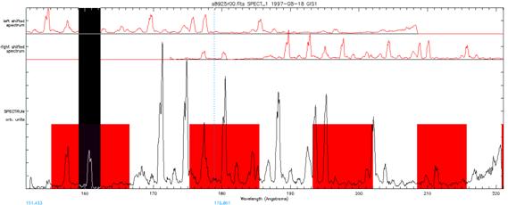
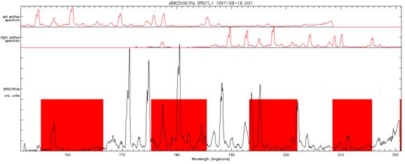
Figure 5: Manual relocation of ghosts using ghost_buster in automatic mode. (top) the region around the ghosted line located at 160? has been selected, and (bottom) relocated to its parent line at 175 ?.
Let go of the mouse and enter r in the terminal window to move the line to the right. Repeat this procedure until all the lines of interest have been corrected. When moving a ghost, remember to include enough background for line fitting on either side of the line of interest. It is possible to restore more ghosts by running the program again, on the same detector or any other. Use the /plot or /hardcopy keywords to see the final result; alternatively use gis_plot or ghost_plot_one when finished. 4.3.3 Saving and restoring ghost_buster sessions By adding the save = save_struct keyword, it is possible to save the ghost corrections made in manual mode into an IDL structure variable. It is then possible to restore these corrections to uncorrected data with
For example:
and then at a later time
The first call to ghost_buster is in manual mode, and the software will prompt for corrections to the data as outlined above. The corrections are stored in an IDL save file. The second call uses the restored information to reapply the corrections to a second data set. Note that both qlds1 and qlds2 must use the same GSET; and that the same detector (number 1 in this case) must be used. 4.4 Edge effects Most detectors show edge effects, both as spikes and a gradual increase in the background. There are many causes for these effects, notably: a compression of the wavelength scale, causing an increase in the background; end spoiling in the microchannel plates, where the strong electric fields diverge at the ends of the detectors; changes in the solar background, mainly from the HeII continuum; and some very bright (solar) lines, seen especially in detector 2. Preliminary corrections for the non solar sources are now included in gis_calib. These have relatively large errors associated with them (which are passed into the output structure). These will reduce as we acquire more observations to check the corrections. 5. Calibrating GIS Data The GIS calibration has recently been updated using the results of workshops which were held at the International Space Science Institute (ISSI) during 2001. These workshops were used to determine (using intercalibration observations) to find an absolute and relative intensity calibration for all the instruments on SOHO. This resulted in an overall upward shift in the sensitivity of the GIS by 2.6. More recently it has been found that the lines in GIS 1 and 2 were becoming degraded due to the effects of Long term gain depression. For this reason new flat field files have been generated to correct for this degradation. Because of the size of the corrections (as much as 60%) and associated uncertainty, a pixel by pixel error array is now included in the calibrated qlds structure. This can be extracted using the gis_error function
Wavelength calibrations are read in automatically when the fits file is converted to a qlds. The wavelength calibration can be accessed by the routines wave2pix, pix2wave, which translate the GIS pixel co-ordinates as necessary.
Where, for the GIS, spec_id is a string containing GIS1 GIS2 GIS3 or wavelength can be a single value or an array. See the example program B. Similarly
Which will return the wavelengths of the pixel array for the spectrum. Again, the input can be a single value or an array. Variations of about 20% of a line width are expected between observations, caused mainly by GIS hardware temperature differences when observing different areas of the sun, or very high count-rates (more than about 40 counts/second/pixel) causing distortions in the electronic processing. Note that the wavelength calibration varies with each GIS setup (GSET) compare two GIS observations that used different GSETs it is necessary wavelength calibration. This is simplified with the routine restore_wavecal. For instance, below is part of an IDL session to over plot two GIS observations:
As well as the ghosts and fixed patterning, the detectors and their electronics have non-linearities that need to be corrected. On the whole these corrections are small (less than 10%, but dependent on count-rate). gis_calib will correct for these (as well as correct for gain depression); and calibrate from counts into photons using the updated GIS calibration coefficients.
By default the data will be returned in calibrated units of photons/sec/arcsec2/cm2.To convert to photons per second per solid angle per area use the /steradian_m2 or (to leave in counts) /counts switches. The routine checks to make sure the routine ghost_buster has been run for all the detectors - if not the error for data in the regions likely to ghost is set to 100% of the counts in the adjacent arms. Similarly, the error for regions which cannot be calibrated for any other reason is also set; this might include the occasional strong line that is too bright for the gain depression calibration (such as the HeII 304 line), or whole detector count rates too high for the electronic dead time corrections.
The GIS calibration coefficients used are those from the results of the SOHO radiometric inter-calibration workshops which were held at the International Space Science Institute (ISSI) during 2001. The coefficients can be viewed using the program gis_write_calib.
The corrections and calibrations made by gis_calib include:
These routines will work with all storage schemes used for CDS qlds data. With GIS data, specify the qlds and the `window', which is one less than the detector number.
For example, to extract detector 3 data from a pre-defined qlds use
The returned data are a floating point array of up to 4 dimensions: spectrum (always 2048 pixels for the GIS), solar x, solar y, and time. The time dimension is only used for data that have multiple exposures at the same solar x, y point. To get information about the extracted data use
For example:
The returned structure tells us which units the data use (GIS3desc.units), the missing data flag (GIS3desc.missing), the wavelength range (GIS3desc.wavemin, GIS3desc.wavemax), etc. The command
will display all the information available in the structure. Also available is gt_spectrum, to get individual spectra from a raster:
Where window, yix, xix, tix are the user supplied window (i.e., the detector number-1), and for each raster position the x, y and time indices. The time index is not normally used unless the raster has repeated exposures at the same position. If supplied, lambda will return the wavelength for each pixel in the spectrum, xsolar and ysolar are the locations on the sun in arc seconds from the sun centre and time is the time of the start of the exposure.
where wavescale and data are the X and Y variables, waverange can be used to limit the fit to a particular line, and k is the polynomial order of the background. Thus to fit a Gaussian plus background to a region in the first exposure of the above GIS detector 3 data:
Another routine, cds_gauss, has been developed for use with CDS data:
Where x is the independent vector; y is dependent variable; a contains the returned coefficients and k defines the order of the polynomial to be fitted to the background. A more complicated but very comprehensive fitting routine is cfit
Where x, y are the data to be fitted, a is an array of (nominal) parameter values - if defined then used as an initial guess to the fit; fit is a structure containing one tag for each component in the fit; sigma contains the errors for each of the parameter values in a. For detailed information about cfit see CDS software note 47 - The Component Fitting System for IDL.
This routine works on calibrated and uncalibrated data. Un- calibrated data is corrected and calibrated automatically using the individual routines described in the previous sections of the analysis guide (Gis_smooth, Ghost_buster, gis_calib etc). The visible identified lines are then fitted, using the cfit line fitting routine. The output structure contains the fitted line positions, widths, intensities, errors, and total line counts in photons/sec/arcsec2, along with ancillary data such as the location and time of observation. The gisfit structure can be used to quickly produce light curves, images and DEM maps
This plots a time series of the raw accumulated counts for the
selected detector (see Figure 6).
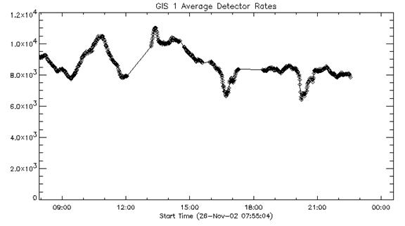
Figure 6: The output from gis_utplot, for a series of sit and stare observations in an active region located at the limb. Note the dimming periods around 17:00 and 20:00 UT. This is investigated in Figure 7 where individual lines are plotted.
This routine also works with arrays of qlds structures. So if you have a series of qlds from a particular observation you can combine these in the following way:
Or alternatively a string array of program numbers for example:
This will read, correct, calibrate and then plot the data, In this case from a sit and stare observation which is displayed in Figure 6. The calibrated and fitted data is saved into the gisfit structure if this variable is passed on the command line. If it already exists it is updated. The gisfit structure can then be used to plot the corrected, calibrated and fitted lines from the observations.
Calling gis_utplot in this fashion will result in a prompt for you
to select a particular line from a list of available present in
the structure to plot. Alternatively, the specific line id can be
entered.
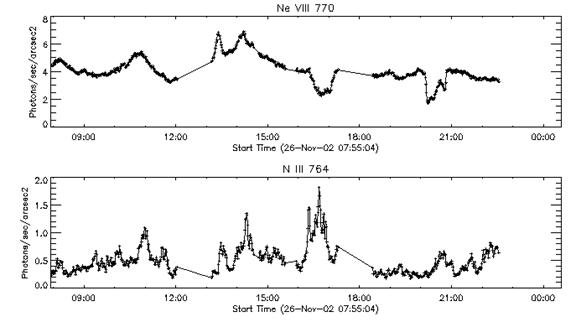
Figure 7: Output from gis_utplot, for specific lines contained in the gisfit structure.
GIS specific software for determining, temperatures, emission measures, densities, and DEM's, based on the output gisfit structure, are under development. To find the latest routines, browse using