XMM RPS Users' Manual

   
Preparing an XMM observation

As described above, preparing XMM observations starts with a technical feasibility calculation, using primarily the information provided in the XMM Users' Handbook (online version: UHB) and the tools introduced there.

  

Figure 1: Preparing an RGS observation using the High Time Resolution (HTR) mode, with an exposure time of 23.6 ks. The RGS observation is assumed to be the science driver of the observation; therefore, it is prepared first and determines the length of the observation.

The scientific goal of the proposal determines the choice of prime science instrument and the total integration time required. It is expected that in all cases either EPIC or RGS will be the most important instrument for the proposed science, i.e., the instrument driving the feasibility calculations (even if, in order to centre the zeroth order image of a source properly in a small OM fast mode window, OM should formally be declared ``primary''). Having determined the total integration time needed for the primary instrument, one must consider in which mode they want this instrument to be operated and how many exposures (possibly in different modes) should be taken during the intended observation. Then the use of the other instruments is planned, which will be operated in parallel.

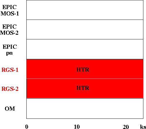
We illustrate this in the following with an example: an RGS HIGH TIME RESOLUTION mode (HTR) observation of a variable X-ray source, let's say, with the aim to monitor its X-ray (and, in parallel, optical/UV) variability over a time period of 23.6 ks (i.e., about six and a half hours; Fig 1).

  

Figure 2: In most cases, the EPIC cameras will run parallel to primary RGS observations, with one exposure covering the entire duration of the observation. Thus, only one exposure each must be entered for the three EPIC instruments. The choice of EPIC operation mode depends primarily on the target's X-ray brightness.

RGS HTR observations should always be accompanied by a SPECTROSCOPY mode exposure to locate the incident spectrum on the CCD chips. However, such an exposure is added automatically by the SOC. Users therefore do not need to consider this at all.

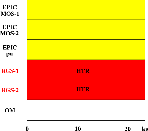
Then one can prepare parallel EPIC exposures. Assuming that there are no special requirements for this observation, in almost all cases only one exposure per instrument is necessary. This is shown in Fig. 2. The only entries that must be made for each EPIC exposure (besides the exposure time) are the choice of EPIC filters for blocking optical light and the operating mode.

Once the X-ray observations are defined, users can start thinking about how to make the best use of OM's capabilities. First it must be checked whether there are any bright stars within the OM FOV. In case of the presence of a bright source (see UHB Table 19 for the limits for all OM optical elements ) the source must either be placed outside the OM FOV by offset pointing XMM or OM must be put in the blocked filter position, ``GO-OFF''. In case simultaneous OM observations are possible in parallel to the X-ray observations, proposers are strongly encouraged to make use of OM's default configurations because of the instrument's inherent complexity (see § 5.3.3.5)! Let us assume that in the present example the observer would be interested in parallel OM imaging mode observations, with RGS-1 as the primary instrument. The OM observations could then be prepared in the following fashion:

  

Figure 3: Parallel to the X-ray observations, OM exposures can now be prepared, using integration times and filter sequences determined as described in the text.

1.

First decide in which OM modes the observations should be carried out (details on this can be found in § 5.3.3.5 and references therein). In the present example, the choice would be ``RGS 1 IMG''.

2.

Then decide upon the choice of OM filters . The recommendation is: U, UVW1, B, UVW2 (see UHB section on OM default configurations ).

3.

Next, consulting UHB Table 14 , choose the correct order of filter sequence. Throughout the observation filters with increasing filter wheel positions must follow each other so as to minimise the wear and tear on the OM's mechanical parts. In the present example, this is: U, B, UVW1 and UVW2 (at filter wheel positions 3, 4, 7 and 9; see UHB section on OM optical elements ).

4.

Then, based on the relative OM filter throughput as shown in UHB Fig. 69 , decide upon the optimal exposure time. The recommended OM exposure time is 1000 s. In the present example, 800 s were chosen for both the B and U filter, 1000 s for UVW1 (because of the lower throughput) and 2120 s for UVW2, which has by far the lowest throughput of the four filters. In this way, similar limiting magnitudes can be reached with all filters.

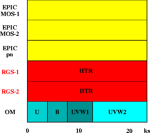For OM default configuration observations the exposure time limits tabulated in § 5.3.3.5 apply.

5.

If, as recommended, a default mode has been chosen, 5 science windows are defined, which will be observed in 5 consecutive exposures, each with the specified exposure time. Thus, each default mode observation takes five times the ``exposure time'' specified by the XRPS user. (Mosaicing later the five science windows, there IS - technically speaking - only one exposure, covering 92% the OM FOV). Therefore, the times for each filter are 4 ks (= $5\times800$ s), 4 ks, 5 ks and 10.6 ks, summing up to 23.6 ks (matching the RGS exposure time).

This leads to the sequence of default mode exposures depicted in Fig. 3. More details on the required inputs will follow in appropriate sections of § 5.

One of the science goals of XMM is to conduct serendipitous surveys. To achieve this, all XMM science instruments should be operating whenever permitted by constraints (such as, e.g., visibility constraints, target brightness, etc.). This implies that exposures should be defined for each instrument for the entire duration of an observation, as demonstrated above.