
| Data Deconvolution for MOSES |
|---|
This web page gives a very brief explanation and assessment of the quality of the MOSES data deconvolution. Hyperlinks are provided for more detail.
Why MOSES ?
MOSES (Multi Order Solar EUV Spectrograph) is a soon to be launched rocket experiment testing the concept of slitless multi-order spectroscopy. The idea is to obtain measurements of a spectral line over an x,y plane on the Sun, i.e. a λ,x,y data cube, with one single exposure. In data cubes obtained with slit scans, as done with CDS or SUMER, different slices of the cube are observed at different times, making the interpretation of time varying phenomena cumbersome. MOSES avoids this problem.
 MOSES data
products and data cube reconstruction
MOSES data
products and data cube reconstruction
The product of a MOSES observation are three images: one image per spectral order n=0, n=-1, and n=+1. The n=0 image is a plain image, integrated over the wavelength range MOSES sees (thus, MOSES is also an imager). The n=+1/-1 images contain spectral information. However, since MOSES is a slitless spectrograph, the dispersion axis coincides with one of the spatial axes (hereafter defined the x-axis). The three MOSES images and an estimate of the average line profile (which corresponds to an infinite order spectrum) are used to reconstruct the original λ,x,y data cube using the Fourier Backprojection Method.
Simulation and quality of data reconstruction
In order to demonstrate the quality of the data deconvolution, we calculate the three images MOSES would observe based on given CDS and SUMER input data cubes, perform the data cube reconstruction, and compare this with the CDS/SUMER input.
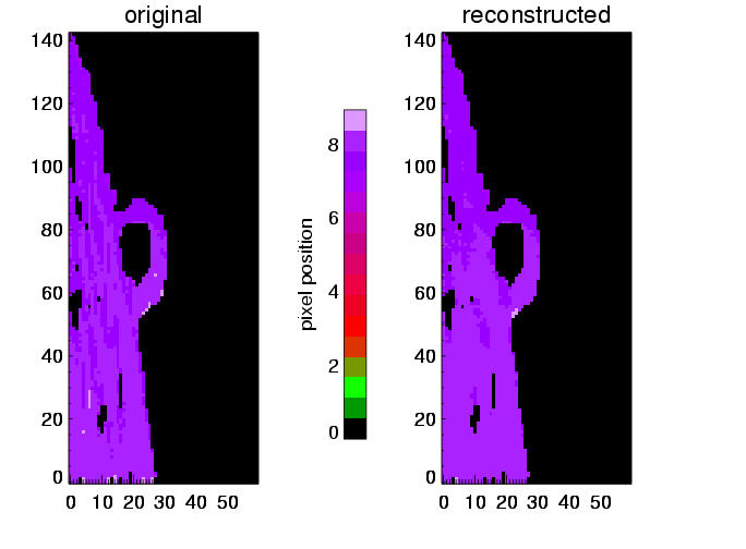
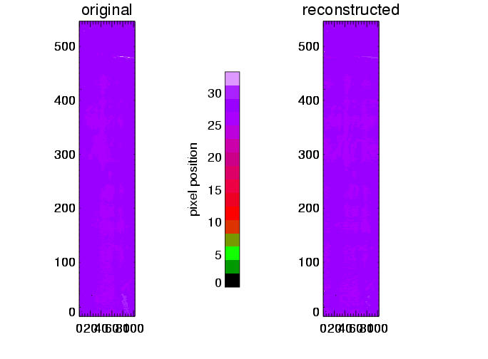
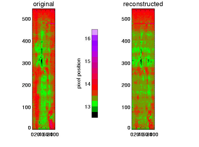
| CDS OV | SUMER NeVIII | SUMER NeVIII, binned in λ |
|
|---|---|---|---|
| maps of line centers, left: from original data cubes, right: reconstructed |
 |
 |
 |
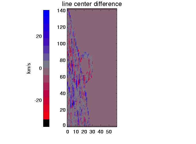
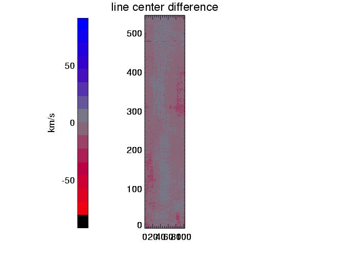
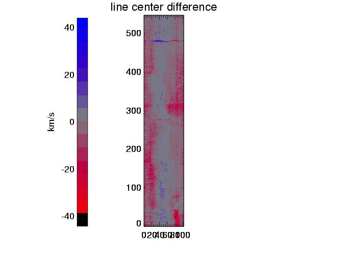
| subtraction of above maps, showing difference between reconstructed and true line centers |
 |
 |
 |
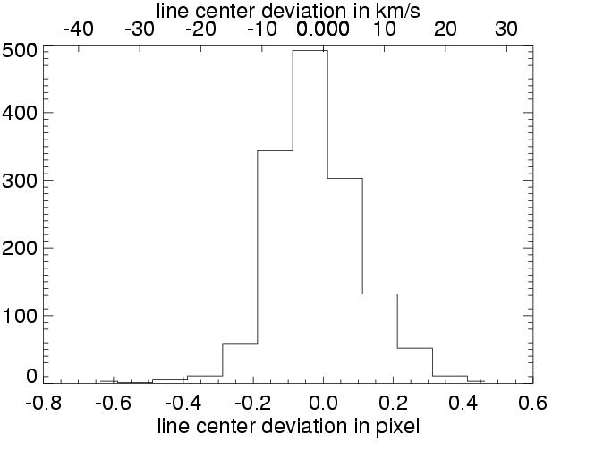
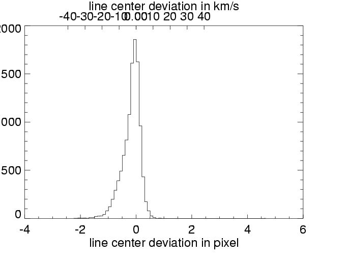
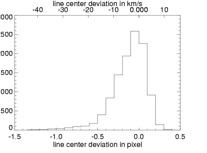
| as above, in histogram |
 |
 |
 |
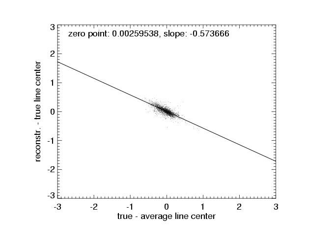
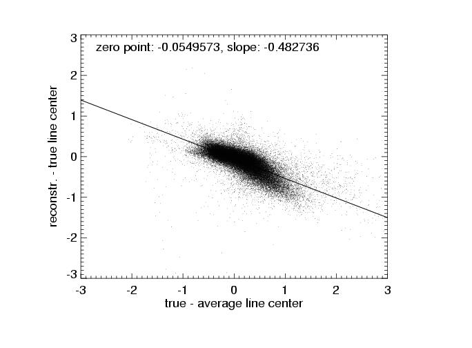
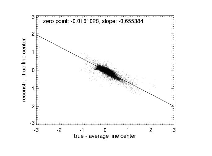
| true - aver. line center vs. true - reconstr. line center |
 |
 |
 |
The above plots show results for three different simulations (columns). The line center maps in the first row - from the original data on the left hand side and from the reconstructed data on the right hand side - show a general agreement between the reconstructed and original data. This becomes clearer in the second row, where the difference of these maps is plotted, and even more suggestive in the third row, where the line center differences between original and reconstruction for all pixels are summarized in a histogram. These histograms would ideally carry all values in the zero bin, but show instead a distribution around zero with a full width of half maximum of approx. 15 to 20 km/s. This value of 15 - 20 km/s in radial velocity can be regarded as the error added to the data by the data reconstruction. The error seems independent of the spectral dispersion (unless the dispersion results in errors greater than 15-20 km/s), and is determined by the number of orders ( = 4) involved in the reconstruction process.
The errors are, however, not perfectly random. The fourth row shows plots of the difference of the true (input) and average line center vs. the difference of the reconstructed and true line center. The distribution of data points can be fitted with a linear relation and shows that the reconstruction tends to pull the line centers to the average value. This is to be expected, as each projection pulls the result towards itself with equal force. Ideally, the distribution of points in these diagramms should have a zero slope.
Work in Progress
More simulations, also with artificial data, will be performed. If the linear relation as shown in row 4 of the table turns out to be unique or similar for all different kinds of test data, then we have the possibility to correct the line center determination and minimize systematic errors. Results will be shown on this web page.
Introduction to Multi-Order Imaging
Wavelength Selection for Solar Orbiter EUI
Detailed Theoretical Information