
| The Fourier Backprojection Method |
|---|
 The Fourier Slice Theorem
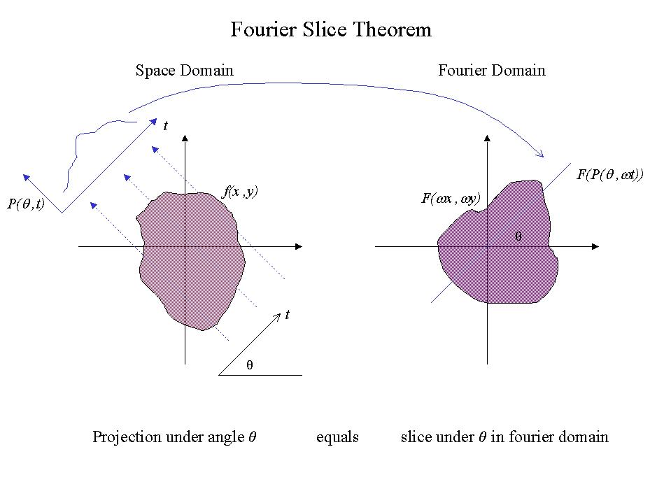
The Fourier Slice Theorem states that the Fourier transform of a projection of a function f(x,y) (1), seen from an angle θ, equals the slice of the fourier transform of f(x,y), F(f(x,y)) = F(ωx, ωy), under that angle θ.
Under the projection we understand the function P(θ, t) which results from integrating along all parallel lines perpendicular to a line (x, y) = t * (cos(θ), sin(θ)) through the origin of the coordiante axes and forming the angle θ with the x-axis.
For details, see the book of A.C. Kak and Malcolm Slaney, "Principles of Computerized Tomographic Imaging", IEEE Press, 1988", also available online at http://www.slaney.org/pct/.
It is clear that if projections from all angles 0 <= θ < π are given, their fourier transforms will completely cover the fourier transform of the function f(x,y). Thus, the function f(x,y) can be determined by its projections when assembling the fourier transforms of the projections correctly and then back-transform to the space domain. A standard application is the mapping of internal body tissue, where X-ray images as projections of, for instance, a tumour, are used to reconstruct a three dimensional image of the tumour itself.
 Fourier Backprojection with MOSES
In the case of MOSES, the three observed orders n=0, -1, +1 and the guessed infinite order (average spectrum) are projections in the above sense of the λ,x plane. Note that the n=+1 and n=-1 orders are indeed independent images as the orientation of x is different relative to λ. The fourier transforms of these four images define four slices in the fourier transform of the λ,x,y data cube.
It is obvious that with only four projections most of the fourier plane remains undefined. These areas are set to zero. As a result, the back-transform results in an image containing many negative intensity values which are physically not meaningful. They are set to zero, and the image is transformed back into the fourier domain. Now, the fourier transform will have values different from zero in those areas which were not defined by the projections. Moreover, some values along the slices defined by the projections will have changed as well. Their values are restored. (2) This will form a second iteration of the fourier image, and it's back transform to the space domain results in a restored λ,x,y data cube with less negative intensity values than in the first iteration. The process is repeated, and after typically a few hundred iterations, the number of negative intensity values is minimzed. Click here for a movie visualizing this process.

 Without the guess of the average line profile as a fourth projection, the
problem would be a bit ill-defined for a good reconstruction. However, when
restricting to the observation of one line, this guess does not pose much of a
problem. Since many spatial pixels and thus many profiles enter the average,
the average profile is close to gaussian. The intensity of the average profile
follows from normalization with the other three observed orders, as all orders
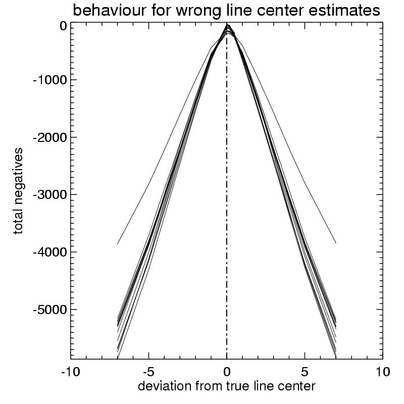
have the same total intensity. Line center and width can be estimated from the
convergence behaviour of above described iteration: if a guessed parameter
differs from the true value, the reconstruction converges to a solution with
more negative intensity values. This is demonstrated in the figures to the
right which show the final (after 1000 iterations) total number of negative
intensity vs. the difference in guessed and true line center and line width,
respectively.
Without the guess of the average line profile as a fourth projection, the
problem would be a bit ill-defined for a good reconstruction. However, when
restricting to the observation of one line, this guess does not pose much of a
problem. Since many spatial pixels and thus many profiles enter the average,
the average profile is close to gaussian. The intensity of the average profile
follows from normalization with the other three observed orders, as all orders
have the same total intensity. Line center and width can be estimated from the
convergence behaviour of above described iteration: if a guessed parameter
differs from the true value, the reconstruction converges to a solution with
more negative intensity values. This is demonstrated in the figures to the
right which show the final (after 1000 iterations) total number of negative
intensity vs. the difference in guessed and true line center and line width,
respectively.
(1) This
applies for any dimension greater or equal than 2. We consider the two
dimensional case of a function dependend of two variables.
(2) Before restoring the fourier transforms of the projections, a low pass
filter is applied in order to surpress high frequency artefacts.
Introduction to Multi-Order Imaging
Wavelength Selection for Solar Orbiter EUI
Detailed Theoretical Information