test_centerhisto.eps		difference of true and reconstructed line center in a histogram
test_centerhisto.dat		histogram data
test_centerhisto_corr.eps	difference of true and corrected reconstructed line center (2)
test_centerhisto_corr.dat	histogram data
test_widthhisto.eps		difference of true and reconstructed line width in a histogram
test_widthhisto.dat		histogram data

test_centermap.eps		map of true (left) and reconstructed (right) line center
test_centermap_corr.eps		map of true (left) and corrected reconstructed (right) line center (2)
test_centerdiffmap.eps		map of line center differences
test_centerdiffmap_c.eps	map of line center differences for corrected line centers (2)

test_widthmap.eps		map of true (left) and reconstructed (right) line widths
test_widthdiffmap.eps		map of line width differences

test_image.eps			map of true (left) and reconstructed (right) intensities for the 
				wavelength point of maximum intensity

For illustration, here are the graphic results for the line center reproduction of this examples, i.e. the files test_centermap.eps, test_centerdiffmap.eps and test_centerhisto.eps (from left to right):

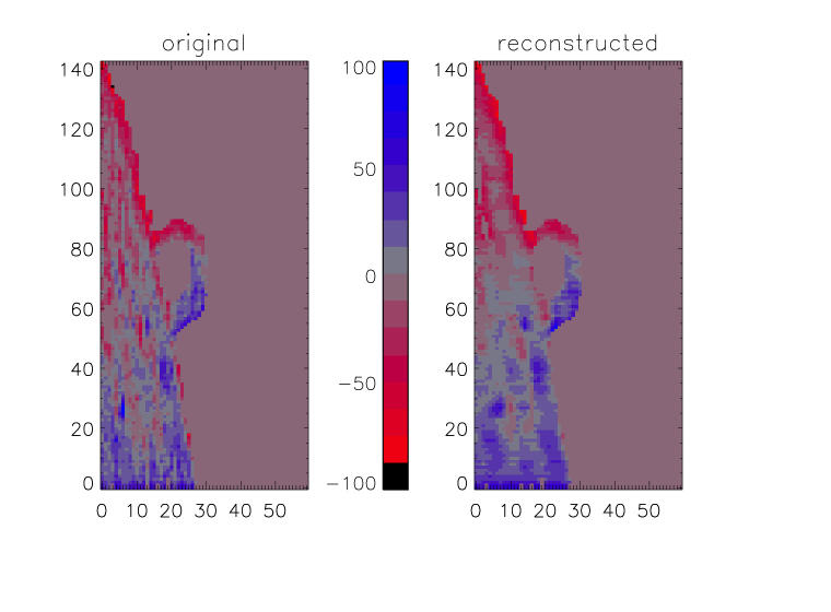
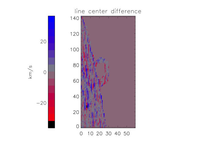
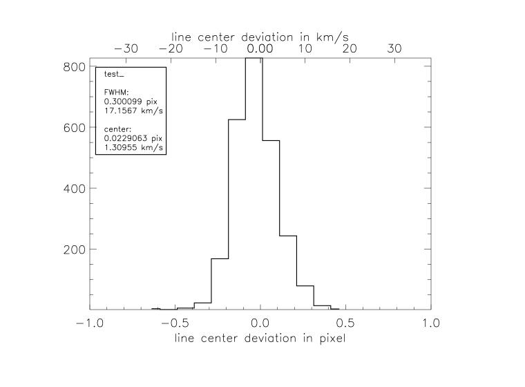
The images should be self-explanatory. Finally, the procedure parametertrend.pro investigates the systematic error seen in reconstructed line centers:

IDL> parametertrend, "test_"

The only neccessary argument is the file prefix string. The procedure plots the difference between the true line center λ (known from the input data cube) and the line center of the average profile of the corresponding image slice, λ_av, vs. the difference between the reconstructed line center λ_re and the true line center λ into a postscript file test_trend.eps. Such a plot looks like this:

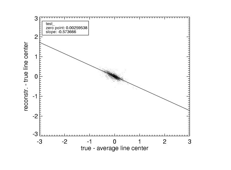
The procedure also performs a linear fit to the cloud of points in this diagram:

(λ_re - λ) = A + B(λ - λ_av)

Ideally, the point cloud would not extend along the y-axis at all, meaning that the reconstructed line center agrees for all pixels with the input value. With only random errors resulting from the reconstruction, the point cloud will have some vertical scatter, but in such a sense that a linear fit has still zero slope B and zero point A=0 (i.e. runs horizonally and through the origin). The latter turns out to be true, but the slope is not zero, pointing at a systematic error in a sense that the reconstructed line centers are underestimated and pulled towards the average value. This is a direct consequence of the fact that the data cube reconstruction is performed with only 4 projected images (three spectral orders and average line profile). One can imagine the average line profile to pull the result towards itself, thus causing an underestimation of the individual line centers. It is the average data of such linear fits, performed on many test images, which could provide a correction factor for the line center reproduction. The average fit parameters enter the code in the procedure prepgraphics.pro. Unfortunately, it turnes out that the slope of above fits is not unique for all possible test images but depends on the image itself. That is why the graph test_trend_c.eps, which shows the same as test_trend.eps but with the correction applied, does not show a point cloud with zero slope (see also footnote 2). The correction factor hardwired in prepgraphics.pro will have to be changed when a suitable correction has been found.

For the sake of completeness, the procedure paramtertrend.pro performs the same analysis on the line widths, so that the files created by the procedure are:

test_trend.eps
test_trend_c.eps
test_trendw.eps

Moreover, zero point and slope of the fits are printed on the terminal window:

test_ center -      fit zeropoint, slope:    0.00259538    -0.573666
test_ corr.center - fit zeropoint, slope:     0.0102484    -0.312289

Again, in the ideal case, the numbers in the last row should both be zero.

Miscalleneous

The Perl script eps2jpg transforms encapsulated postscript files to jpeg format and creates an icon sized picture which comes in handy for html documents:

./eps2jpg file.eps

The files created are called file.jpg and file_icon.jpg. The script can also run on a file filelist containing a list of .eps files:

./eps2jpg -file filelist

So a quick way to create jpegs and icons out of all .eps files would be

ls *.eps > temp

./eps2jpg -file temp

The script mkhtml uses the html template restemplate.html and produces a file test_result.html serving as a quick-look html file displaying the most interesting graphs. If more than one test run results should be displayed on the same web page, mkhtml can take a file containing a list of prefixes:

./mkhtml -file list

(1) the software is not designed for multiple emission line spectra, but for single line profiles only. For multiple line spectra, the replacement of the average spectrum by a gaussian profile should be extended to fit all lines. When applying the simulation to a multiple lined spectrum, only one line will be considered and the others will be ignored. This leads to an overestimation of the lines intensity, since the corresponding overlappogram is normalized in respect to the other three (orders 0, 1, and -1) overlappograms.

(2) an average value of such correction factors is already hardcoded in prepgraphics.pro and the reason for output files with the appendix string "_c" or "_corr" in parallel to all other file output. However, a good correction factor has not yet been found, and probably won't be found as a unique factor since it depends somewhat on some global property of the image. How to correct systematic errors in line centers is still being investigated.